Darunavir (Stillemans 2021)
Source:vignettes/articles/Stillemans_2021_darunavir.Rmd
Stillemans_2021_darunavir.RmdModel and source
- Citation: Stillemans G, Belkhir L, Vandercam B, Vincent A, Haufroid V, Elens L. Exploration of Reduced Doses and Short-Cycle Therapy for Darunavir/Cobicistat in Patients with HIV Using Population Pharmacokinetic Modeling and Simulations. Clin Pharmacokinet. 2021;60:177-189. doi:10.1007/s40262-020-00920-z. PMCID: PMC7862523.
- Description: One-compartment population pharmacokinetic model with first-order absorption and elimination for oral cobicistat- or ritonavir-boosted darunavir in adults with HIV-1 infection (Stillemans 2021). Apparent clearance decreases exponentially with alpha-1 acid glycoprotein (AAG), is lower in women and in CYP3A5 nonexpressers (3/3); apparent volume decreases exponentially with AAG and is higher in SLCO3A1 rs8027174 G>T carriers.
- Article: https://doi.org/10.1007/s40262-020-00920-z (open access, PMC7862523)
- Electronic supplementary material (covariate-selection table used for the equation forms): Online Resource 2 of the article.
The model is a one-compartment model with first-order absorption and first-order elimination for oral darunavir boosted with cobicistat (most patients) or ritonavir. Apparent clearance (CL/F) falls exponentially with plasma alpha-1 acid glycoprotein (AAG), is lower in women and in CYP3A5 nonexpressers (3/3); apparent volume (V/F) falls exponentially with AAG and is 81% larger in SLCO3A1 rs8027174 G>T carriers.
Population
The model was fitted to 405 darunavir concentrations from 127 adults with HIV-1 infection followed at the Cliniques Universitaires Saint-Luc, Brussels (NCT03101644): 309 sparse samples taken at random post-intake times during routine visits, plus 96 samples from 12-hour rich profiles (pre-dose to 6 h) in 12 adherent patients (Methods 2.1, Results 3.1). Median age was 55 years (IQR 13), median weight 73 kg (IQR 17), 33.1% were women, 52.8% Caucasian and 43.3% African. Most patients took darunavir 800 mg once daily (91.3%); 85.8% were boosted with cobicistat and 14.2% with ritonavir (Table 1). CYP3A5 genotypes were 1/1 26.0%, 1/3 26.0% and 3/3 45.7%; 14.2% carried the SLCO3A1 rs8027174 T allele and none were T/T (Table 2).
The same information is available programmatically:
str(rxode2::rxode(readModelDb("Stillemans_2021_darunavir"))$population)
#> ℹ parameter labels from comments will be replaced by 'label()'
#> List of 13
#>  $ species       : chr "human"
#>  $ n_subjects    : num 127
#>  $ n_studies     : num 1
#>  $ n_observations: num 405
#>  $ age_median    : chr "55 years (IQR 13)"
#>  $ weight_median : chr "73 kg (IQR 17)"
#>  $ sex_female_pct: num 33.1
#>  $ race_ethnicity: chr "Caucasian 52.8%, African 43.3%, other 3.9% (Table 1)"
#>  $ disease_state : chr "HIV-1 infection, adult outpatients on boosted darunavir (median treatment duration 4.2 years; 78.7% with viral "| __truncated__
#>  $ dose_range    : chr "darunavir 800 mg q24h (91.3%), 600 mg q12h (7.9%) or 1200 mg q24h (0.8%); boosted with cobicistat (85.8%) or ritonavir (14.2%)"
#>  $ regions       : chr "Belgium (Cliniques Universitaires Saint-Luc, Brussels)"
#>  $ genotypes     : chr "CYP3A5 *1/*1 26.0%, *1/*3 26.0%, *3/*3 45.7%; SLCO3A1 rs8027174 G/T 14.2% (Table 2)"
#>  $ notes         : chr "Prospective observational TDM study (NCT03101644). Dataset A: 309 sparse samples, one per visit at random post-"| __truncated__
Source trace
Every ini() value carries an in-file comment naming its
source. The table collects them.
| Equation / parameter | Value | Source location |
|---|---|---|
| One-compartment, first-order absorption and elimination, no lag | n/a | Results 3.2 |
lka (ka) |
log(0.68) 1/h | Table 3 |
lcl (CL/F) |
log(12.9) L/h | Table 3 |
lvc (V/F) |
log(152) L | Table 3 |
e_aag_cl |
-0.61 per g/L, exponential | Table 3; equation form Methods 2.6 and ESM Online Resource 2 |
e_aag_vc |
-0.68 per g/L, exponential | Table 3; ESM Online Resource 2 |
e_sexf_cl |
-0.21, exponential | Table 3; ESM Online Resource 2 |
e_cyp3a5_cl |
-0.16, categorical on nonexpressers | Table 3; ESM Online Resource 2; Results 3.3 (‘19% higher in expressors’) |
e_snp_slco3a1_rs8027174_vc |
0.81, categorical | Table 3; ESM Online Resource 2; Results 3.3 (‘increased by 81%’) |
etalka |
0.60^2 = 0.36 | Table 3, ‘omega ka (SD)’ |
etalcl |
0.22^2 = 0.0484 | Table 3, ‘omega CL (SD)’ |
etalvc |
0.33^2 = 0.1089 | Table 3, ‘omega V (SD)’ |
propSd |
0.281 | Table 3, ‘sigma exponential (SD)’ |
addSd |
0.641 mg/L | Table 3, ‘sigma additive (SD)’ |
| AAG centring value | 1 g/L (assumed) | Not reported; see Assumptions |
The covariate equations are those printed in Methods 2.6, with the form for each retained covariate taken from ESM Online Resource 2:
- Exponential:
P = theta * exp(theta_cov * (cov - median))(AAG on CL/F and V/F; sex on CL/F, with male as the reference so the female term isexp(-0.21)). - Categorical:
P = theta * (1 + theta_cov)for the non-reference group (CYP3A5 nonexpressers on CL/F; SLCO3A1 T carriers on V/F).
Typical-value covariate effects
These are deterministic properties of the model file and are checked against the paper’s own statements.
ui <- rxode2::rxode(readModelDb("Stillemans_2021_darunavir"))
#> ℹ parameter labels from comments will be replaced by 'label()'
th <- ui$theta
typical <- tibble::tribble(
  ~Effect, ~Model, ~Paper,
  "CL/F expresser / nonexpresser", 1 / (1 + th[["e_cyp3a5_cl"]]), 1.19,
  "CL/F female / male", exp(th[["e_sexf_cl"]]), exp(-0.21),
  "V/F SLCO3A1 T carrier / G/G", 1 + th[["e_snp_slco3a1_rs8027174_vc"]], 1.81,
  "CL/F at AAG + 1 g/L / at centre", exp(th[["e_aag_cl"]]), exp(-0.61),
  "V/F at AAG + 1 g/L / at centre", exp(th[["e_aag_vc"]]), exp(-0.68)
)
knitr::kable(typical, digits = 3, caption = "Typical-value covariate ratios.")| Effect | Model | Paper |
|---|---|---|
| CL/F expresser / nonexpresser | 1.190 | 1.190 |
| CL/F female / male | 0.811 | 0.811 |
| V/F SLCO3A1 T carrier / G/G | 1.810 | 1.810 |
| CL/F at AAG + 1 g/L / at centre | 0.543 | 0.543 |
| V/F at AAG + 1 g/L / at centre | 0.507 | 0.507 |
Virtual cohort
The observed data are not public. Table 4 of the paper was produced by simulating steady-state profiles for the study cohort itself (1000 replicates, no residual error) under each of four regimens, so every regimen saw the same patients. The virtual cohort mirrors that: 200 patients whose covariate frequencies follow Tables 1 and 2, each with one draw of the random effects, replicated under all four regimens. AAG is not summarised in the paper, so it is drawn from a log-normal distribution centred on the model’s AAG centring value (see Assumptions).
# `set.seed()` seeds R's RNG, which draws both the covariates and the random
# effects here (the etas are supplied as data columns, see below), so the
# cohort is the same on every machine. The assertions are nonetheless
# written with Monte-Carlo headroom rather than to one draw.
set.seed(20210722)

mod <- readModelDb("Stillemans_2021_darunavir")
omega <- rxode2::rxode(mod)$omega
#> ℹ parameter labels from comments will be replaced by 'label()'
stopifnot(all(omega[upper.tri(omega)] == 0))

n_subj <- 200

subjects <- tibble(
  subject = seq_len(n_subj),
  SEXF = rbinom(n_subj, 1, 42 / 127),
  # Expressers (*1/*1 + *1/*3) among genotyped subjects, Table 2
  CYP3A5_EXPR = rbinom(n_subj, 1, 66 / 124),
  # G/T carriers among genotyped subjects, Table 2
  SNP_SLCO3A1_RS8027174 = rbinom(n_subj, 1, 18 / 123),
  AAG = exp(rnorm(n_subj, log(1), 0.34))
)
for (eta in colnames(omega)) {
  subjects[[eta]] <- rnorm(n_subj, 0, sqrt(omega[eta, eta]))
}

regimens <- tibble::tribble(
  ~regimen, ~dose, ~days_on,
  "800 mg q24h", 800, 7,
  "600 mg q24h", 600, 7,
  "400 mg q24h", 400, 7,
  "800 mg q24h 5/7 days", 800, 5
)

make_arm <- function(regimen, dose, days_on, id_offset) {
  subj <- subjects |>
    mutate(id = id_offset + subject, regimen = regimen)
  # Three weeks of dosing; within each week doses on days_on consecutive
  # days. The analysis window is the third week (336-504 h), when the
  # once-daily arms are at steady state (half-life about 10 h).
  dose_times <- as.vector(outer((seq_len(days_on) - 1) * 24, c(0, 168, 336), "+"))
  obs_times <- sort(unique(c(seq(336, 504, by = 1), seq(336, 340, by = 0.25))))
  doses <- tidyr::crossing(subj, time = dose_times) |>
    mutate(amt = dose, evid = 1L, cmt = "depot")
  obs <- tidyr::crossing(subj, time = obs_times) |>
    mutate(amt = 0, evid = 0L, cmt = "central")
  bind_rows(doses, obs) |>
    arrange(id, time, desc(evid))
}

events <- bind_rows(lapply(seq_len(nrow(regimens)), function(i) {
  make_arm(
    regimens$regimen[i], regimens$dose[i], regimens$days_on[i],
    id_offset = (i - 1L) * n_subj
  )
}))
stopifnot(!anyDuplicated(unique(events[, c("id", "time", "evid")])))
Simulation
Table 4 was simulated without residual error, so the comparison uses
Cc (the individual prediction), not the residual-error
sim column. The model is solved with its random effects
zeroed; the per-patient eta columns in the event table then supply each
patient’s random effects, identically in every regimen.
sim <- rxode2::rxSolve(
  rxode2::zeroRe(mod),
  events = events,
  keep = c("regimen", "subject"),
  returnType = "data.frame"
) |>
  mutate(regimen = factor(regimen, levels = regimens$regimen))
#> ℹ parameter labels from comments will be replaced by 'label()'
#> ℹ omega/sigma items treated as zero: 'etalka', 'etalcl', 'etalvc'
#> Warning: multi-subject simulation without without 'omega'

# The eta columns must reach the solve: the same patient's CL/F differs
# between patients but is identical across the four regimens.
cl_by_arm <- sim |>
  distinct(subject, regimen, cl)
stopifnot(
  nrow(cl_by_arm) == 4 * n_subj,
  sd(log(cl_by_arm$cl[cl_by_arm$regimen == "800 mg q24h"])) > 0.15,
  all(tapply(cl_by_arm$cl, cl_by_arm$subject, function(x) diff(range(x))) < 1e-8)
)

# The model is linear, so with shared patients the once-daily troughs scale
# exactly with dose, as Table 4's do (1.17 / 1.56 = 0.75, 0.78 / 1.56 = 0.50).
trough <- sim |>
  dplyr::filter(time == 360, regimen != "800 mg q24h 5/7 days") |>
  select(subject, regimen, Cc) |>
  tidyr::pivot_wider(names_from = regimen, values_from = Cc)
stopifnot(
  max(abs(trough[["600 mg q24h"]] / trough[["800 mg q24h"]] - 0.75)) < 1e-4,
  max(abs(trough[["400 mg q24h"]] / trough[["800 mg q24h"]] - 0.50)) < 1e-4,
  abs(1.17 / 1.56 - 0.75) < 0.01,
  abs(0.78 / 1.56 - 0.50) < 0.01
)
Steady-state profiles
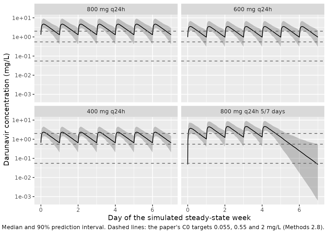
sim |>
  mutate(day = (time - 336) / 24) |>
  group_by(regimen, day) |>
  summarise(
    Q05 = quantile(Cc, 0.05),
    Q50 = median(Cc),
    Q95 = quantile(Cc, 0.95),
    .groups = "drop"
  ) |>
  ggplot(aes(day, Q50)) +
  geom_ribbon(aes(ymin = Q05, ymax = Q95), alpha = 0.25) +
  geom_line() +
  geom_hline(yintercept = c(0.055, 0.55, 2), linetype = "dashed", colour = "grey40") +
  facet_wrap(~regimen) +
  scale_y_log10() +
  labs(
    x = "Day of the simulated steady-state week",
    y = "Darunavir concentration (mg/L)",
    caption = paste(
      "Median and 90% prediction interval. Dashed lines: the paper's",
      "C0 targets 0.055, 0.55 and 2 mg/L (Methods 2.8)."
    )
  )
PKNCA validation
For the once-daily arms the steady-state interval is the last 24 h of
the second week of dosing, 336-360 h (dose at 336 h, trough at 360 h).
For the weekends-off arm the paper takes ‘the C0 immediately before a
new cycle (day 8) and the AUC over day 7 to day 8’ (Table 4 footnote),
i.e. 480-504 h here, 48-72 h after the fifth dose of the week. The
trough is summarised with cmin; within each of these
windows the minimum is the end-of-window concentration.
sim_nca <- sim |>
  dplyr::filter(!is.na(Cc)) |>
  dplyr::select(id, time, Cc, regimen) |>
  mutate(regimen = as.character(regimen))

dose_df <- events |>
  dplyr::filter(evid == 1) |>
  dplyr::select(id, time, amt, regimen)

conc_obj <- PKNCA::PKNCAconc(sim_nca, Cc ~ time | regimen + id)
dose_obj <- PKNCA::PKNCAdose(dose_df, amt ~ time | regimen + id)

intervals <- data.frame(
  regimen = regimens$regimen,
  start = c(336, 336, 336, 480),
  end = c(360, 360, 360, 504),
  cmin = TRUE,
  auclast = TRUE
)

nca_res <- PKNCA::pk.nca(
  PKNCA::PKNCAdata(conc_obj, dose_obj, intervals = intervals)
)
Comparison against Table 4
published <- tibble::tribble(
  ~regimen, ~cmin, ~auclast,
  "800 mg q24h", 1.56, 76.2,
  "600 mg q24h", 1.17, 57.2,
  "400 mg q24h", 0.78, 38.1,
  "800 mg q24h 5/7 days", 0.1, 6.5
)

cmp <- nlmixr2lib::ncaComparisonTable(
  simulated = nca_res,
  reference = published,
  by = "regimen",
  units = c(cmin = "mg/L", auclast = "mg*h/L"),
  tolerance_pct = 20
)
knitr::kable(
  cmp,
  caption = paste(
    "Simulated vs. published (Table 4) median C0 and AUC0-24.",
    "* differs from the published value by more than 20%."
  )
)| NCA parameter | regimen | Reference | Simulated | % diff |
|---|---|---|---|---|
| Cmin (mg/L) | 800 mg q24h | 1.56 | 1.31 | -16.0% |
| Cmin (mg/L) | 600 mg q24h | 1.17 | 0.982 | -16.0% |
| Cmin (mg/L) | 400 mg q24h | 0.78 | 0.655 | -16.0% |
| Cmin (mg/L) | 800 mg q24h 5/7 days | 0.1 | 0.0484 | -51.6%* |
| AUClast (mg*h/L) | 800 mg q24h | 76.2 | 70.3 | -7.7% |
| AUClast (mg*h/L) | 600 mg q24h | 57.2 | 52.7 | -7.8% |
| AUClast (mg*h/L) | 400 mg q24h | 38.1 | 35.2 | -7.7% |
| AUClast (mg*h/L) | 800 mg q24h 5/7 days | 6.5 | 2.9 | -55.3%* |
sim_medians <- as.data.frame(nca_res) |>
  dplyr::filter(PPTESTCD %in% c("cmin", "auclast")) |>
  group_by(regimen, PPTESTCD) |>
  summarise(sim = median(PPORRES), .groups = "drop") |>
  tidyr::pivot_wider(names_from = PPTESTCD, values_from = sim) |>
  inner_join(published, by = "regimen", suffix = c("_sim", "_pub")) |>
  mutate(
    auc_pct = 100 * (auclast_sim / auclast_pub - 1),
    c0_pct = 100 * (cmin_sim / cmin_pub - 1)
  )
daily <- sim_medians |> dplyr::filter(regimen != "800 mg q24h 5/7 days")
stopifnot(nrow(daily) == 3)
# AUC0-24 is the structural check: at steady state it equals dose / CL/F,
# so a mis-transcribed clearance or covariate effect moves it by tens of
# percent. Realised -8% for this cohort (-2% to -4% with 1000-patient
# cohorts in development); 12% leaves room for the Monte-Carlo error of a
# 200-patient median (about 3%).
stopifnot(all(abs(daily$auc_pct) < 12))
# C0 median runs about 15% below Table 4 (realised -16%; see Assumptions and
# deviations); 25% still fails on a halved or doubled volume.
stopifnot(all(abs(daily$c0_pct) < 25))
The once-daily AUC0-24 medians reproduce Table 4 to within about 8%. The simulated median troughs are about 15% below Table 4 and the weekends-off trough and AUC are about half of the published values; both point to the paper’s simulations having a somewhat slower elimination than the Table 3 estimates imply for this virtual cohort (see Assumptions and deviations).
Probability of target attainment (Table 4)
c0 <- as.data.frame(nca_res) |>
  dplyr::filter(PPTESTCD == "cmin") |>
  dplyr::select(id, regimen, C0 = PPORRES)

pta <- c0 |>
  group_by(regimen) |>
  summarise(
    `C0 > 0.055 mg/L` = 100 * mean(C0 > 0.055),
    `C0 > 0.55 mg/L` = 100 * mean(C0 > 0.55),
    `C0 > 2 mg/L` = 100 * mean(C0 > 2),
    .groups = "drop"
  ) |>
  tidyr::pivot_longer(-regimen, names_to = "target", values_to = "Simulated")

pta_pub <- tibble::tribble(
  ~regimen, ~target, ~Published,
  "800 mg q24h", "C0 > 0.055 mg/L", 99.3,
  "800 mg q24h", "C0 > 0.55 mg/L", 89.6,
  "800 mg q24h", "C0 > 2 mg/L", 33.2,
  "600 mg q24h", "C0 > 0.055 mg/L", 99.1,
  "600 mg q24h", "C0 > 0.55 mg/L", 84.0,
  "600 mg q24h", "C0 > 2 mg/L", 16.4,
  "400 mg q24h", "C0 > 0.055 mg/L", 98.6,
  "400 mg q24h", "C0 > 0.55 mg/L", 69.8,
  "400 mg q24h", "C0 > 2 mg/L", 3.6,
  "800 mg q24h 5/7 days", "C0 > 0.055 mg/L", 60.7,
  "800 mg q24h 5/7 days", "C0 > 0.55 mg/L", 15.3,
  "800 mg q24h 5/7 days", "C0 > 2 mg/L", 1.3
)

pta_cmp <- pta_pub |>
  inner_join(pta, by = c("regimen", "target")) |>
  mutate(Difference = Simulated - Published)
stopifnot(nrow(pta_cmp) == nrow(pta_pub))

pta_cmp |>
  dplyr::rename("Regimen" = regimen, "Target" = target, "Published (%)" = Published,
                "Simulated (%)" = Simulated, "Difference (points)" = Difference) |>
knitr::kable(digits = 1, caption = "Probability of target attainment, simulated vs. Table 4.")| Regimen | Target | Published (%) | Simulated (%) | Difference (points) |
|---|---|---|---|---|
| 800 mg q24h | C0 > 0.055 mg/L | 99.3 | 99.5 | 0.2 |
| 800 mg q24h | C0 > 0.55 mg/L | 89.6 | 90.5 | 0.9 |
| 800 mg q24h | C0 > 2 mg/L | 33.2 | 18.0 | -15.2 |
| 600 mg q24h | C0 > 0.055 mg/L | 99.1 | 99.0 | -0.1 |
| 600 mg q24h | C0 > 0.55 mg/L | 84.0 | 84.5 | 0.5 |
| 600 mg q24h | C0 > 2 mg/L | 16.4 | 7.5 | -8.9 |
| 400 mg q24h | C0 > 0.055 mg/L | 98.6 | 99.0 | 0.4 |
| 400 mg q24h | C0 > 0.55 mg/L | 69.8 | 59.5 | -10.3 |
| 400 mg q24h | C0 > 2 mg/L | 3.6 | 1.0 | -2.6 |
| 800 mg q24h 5/7 days | C0 > 0.055 mg/L | 60.7 | 44.5 | -16.2 |
| 800 mg q24h 5/7 days | C0 > 0.55 mg/L | 15.3 | 4.0 | -11.3 |
| 800 mg q24h 5/7 days | C0 > 2 mg/L | 1.3 | 0.0 | -1.3 |
pta_gap <- function(reg, tgt) {
  v <- pta_cmp$Difference[pta_cmp$regimen == reg & pta_cmp$target == tgt]
  if (length(v) != 1L) stop("no unique PTA row for ", reg, " / ", tgt)
  v
}
# 0.055 mg/L on the once-daily arms: nearly everyone is above it in both
# the paper and the simulation (binomial SE under 1 point near 99%).
stopifnot(
  abs(pta_gap("800 mg q24h", "C0 > 0.055 mg/L")) < 5,
  abs(pta_gap("600 mg q24h", "C0 > 0.055 mg/L")) < 5,
  abs(pta_gap("400 mg q24h", "C0 > 0.055 mg/L")) < 5
)
# 0.55 mg/L at 800 and 600 mg: realised within 1 point here; the
# binomial SE at 200 patients is about 2.5 points. The 400 mg / 0.55 mg/L
# and all 2 mg/L cells sit on the steep part of the trough distribution and
# inherit the trough deviation, so they are reported but not gated.
stopifnot(
  abs(pta_gap("800 mg q24h", "C0 > 0.55 mg/L")) < 10,
  abs(pta_gap("600 mg q24h", "C0 > 0.55 mg/L")) < 10
)
# Weekends-off therapy: the paper's conclusion is that it leaves a large
# share of patients below even the lowest target (39.3% below 0.055 mg/L)
# and almost nobody above 2 mg/L. Assert that qualitative result only; the
# magnitude is a known deviation.
sct <- pta_cmp |> dplyr::filter(regimen == "800 mg q24h 5/7 days")
stopifnot(
  sct$Simulated[sct$target == "C0 > 0.055 mg/L"] < 85,
  sct$Simulated[sct$target == "C0 > 2 mg/L"] < 10
)
The once-daily regimens reproduce the 0.055 mg/L target, and the 0.55 mg/L target at 800 and 600 mg, closely. At 400 mg for 0.55 mg/L, and for the 2 mg/L target at every dose, fewer simulated than published patients reach the target, consistent with the lower simulated troughs. For weekends-off therapy the qualitative conclusion is reproduced – a large fraction of patients fall below 0.055 mg/L before the next cycle – but the simulated fractions above each target are lower than in Table 4.
Assumptions and deviations
-
AAG centring value. The paper centres the
exponential AAG effects on the cohort median, but prints that median
nowhere (not in Table 1, the supplement, or the companion
external-validation paper doi:10.1007/s00228-020-03036-2, whose validation data
had no AAG). The model file centres on 1 g/L, a round value inside the
adult reference interval. The typical CL/F and V/F therefore describe a
patient with AAG 1 g/L. If the true median was M g/L, a user-supplied
AAG gives CL/F multiplied by
exp(0.61 * (M - 1))and V/F byexp(0.68 * (M - 1))relative to the published model – about 6% and 7% per 0.1 g/L of difference. Population-level simulations such as Table 4 are unaffected provided the virtual AAG distribution is centred on the same value. - AAG distribution in the virtual cohort. Not reported; drawn log-normal with median 1 g/L and log-SD 0.34 (about 35% CV). The only AAG values the paper prints are two outliers at 2.66 and 2.2 g/L.
-
Sex effect form. ESM Online Resource 2 lists the
sex effect as exponential, so women have CL/F multiplied by
exp(-0.21) = 0.81, i.e. 19% lower; the Results prose says ‘21% lower’, reading the coefficient directly. The printed equation form was followed. -
CYP3A5 coding. The paper’s ’CYP3A53 on CL’
applies to 3/*3 nonexpressers with expressers as reference (‘CL
being 19% higher in expressors’, 1/0.84 = 1.19). The model uses the
canonical expresser column
CYP3A5_EXPRand applies the effect to1 - CYP3A5_EXPR. - Residual error. The paper describes a ‘mixed (additive plus exponential)’ residual model with SDs 0.281 and 0.641 mg/L. It is encoded as proportional plus additive error, the linear-scale equivalent of an exponential term for moderate SDs.
- Covariate frequencies. Missing genotypes (2-3%) were set to the most frequent category in the paper; the virtual cohort uses the frequencies among genotyped subjects.
- Known deviation: troughs and the weekends-off tail. With the Table 3 estimates, the simulated steady-state AUC0-24 matches Table 4 to within about 8% but median C0 is about 15% lower, and in the weekends-off regimen the median C0 72 h after the last dose and the day 7-8 AUC are about half of the published 0.1 mg/L and 6.5 mg*h/L. These quantities are governed by the elimination rate CL/V; the published values imply an effective half-life a few hours longer than this cohort produces. Reading the Table 3 IIV as variances instead of SDs does not remove the gap and worsens the PTA agreement, and the AAG centring value cancels out of the simulation. The paper simulated its own patients’ covariates, including the AAG distribution and the joint distribution of genotype and sex, which cannot be reproduced from the published summaries. The deviation is recorded rather than tuned.
- Related model. The companion paper (Stillemans 2021, Eur J Clin Pharmacol, doi:10.1007/s00228-020-03036-2) re-estimated a version of this model without AAG for external validation; that reduced model is a separate publication and is not part of this file.
- No erratum or correction notice was found for the article (Europe PMC author search, 2026-09-27).