Clobetasol propionate: intravenous PK (Duong 2025)
Source:vignettes/articles/Duong_2025_clobetasolPropionate.Rmd
Duong_2025_clobetasolPropionate.RmdModel and source
mod <- readModelDb("Duong_2025_clobetasolPropionate")
ui <- rxode2::rxode(mod)- Citation: Duong JK, van Dijkman S, Ong G, Marta A, Ceci A, Bonifazi E, Della Pasqua O. (2025). Characterizing local and systemic exposure to clobetasol propionate in healthy subjects and patients with atopic dermatitis. Br J Clin Pharmacol 91(11):3150-3166. doi:10.1002/bcp.70102.
- Article: https://doi.org/10.1002/bcp.70102
- Full text and supplement: https://www.ncbi.nlm.nih.gov/pmc/articles/PMC12569561/
What this model is, and what it is not
Duong 2025 builds a Simcyp (version 22) physiologically based pharmacokinetic (PBPK) model of the potent topical corticosteroid clobetasol propionate (CP). A full-PBPK distribution layer, built and checked on intravenous and oral data (Study A), is coupled to Simcyp’s multi-phase multi-layer MechDermA dermal absorption model. That model was calibrated on topical cream and ointment studies in healthy men, then extended with a skin-barrier-impairment model for lesional and non-lesional skin in atopic dermatitis (AD). The paper’s headline results are simulations of local (stratum corneum) and systemic exposure by formulation, skin condition and treated body-surface area (Table 9, Figure 6).
Simcyp’s whole-body mass-balance equations and its MechDermA skin
model are proprietary and do not appear in the paper. The distribution
layer uses Rodgers and Rowland tissue:plasma partition coefficients with
an optimised Kp scalar of 0.22. Table 6 prints that scalar
and the resulting steady-state volume, but no tissue Kp,
organ volume or blood flow, so the multi-tissue structure cannot be
rebuilt. The paper does report, completely, what the
intravenous disposition needs:
- the in vivo systemic clearance input, 27 L/h (Table 6, “CLIV from Study A”);
- its renal component, 0.12 L/h (Table 6);
- the final model’s steady-state volume of distribution, 2.34 L/kg
(Table 6). The
Kpscalar was optimised so that this matches the observed Study A volume of 164 L (Methods, “Intravenous administration”); - and, in Table 7, the PBPK model’s own predicted half-life and AUC after the 2 mg intravenous dose. These are the answer key for any reduction.
That is enough for a one-compartment intravenous reduction with no fitted parameter. Below, it reproduces the platform’s predicted AUC to within 8% and its half-life to within 20%.
Why the topical arms are not reproduced
MechDermA is a one-dimensional diffusion model. Drug partitions out of an evaporating two-phase vehicle into a “brick-and-mortar” stratum corneum, whose many lipid and corneocyte sub-layers each have their own geometry, hydration and partition coefficients. It then diffuses through the viable epidermis, dermis, a hair-follicle shunt, subcutis and muscle into a local blood supply (Supplementary Figure S2; the equations are in a cited Simcyp reference, not in this paper). The paper prints the drug-specific inputs (Tables 3, 4 and 6) and, for the abdomen site only, the number of stratum-corneum layers and the viable-epidermis and dermis thicknesses (Table 5 footnotes). It does not print:
- the transport equations themselves;
- the per-site skin geometry for the back, thigh, lower leg and arms, which carry most of the applied dose in every whole-body study (Tables S4-S6);
- dermal blood flow, hair-follicle density and geometry, or subcutis and muscle thickness.
These are Simcyp system-database values, and no amount of reading the
paper recovers them. The published outputs (Table 7 and Table 9) are
simulated summaries, not a parameterisation. Fitting a simpler
absorption model to them would make a new model of the maintainers’ own,
not a reproduction of the paper’s. The atopic-dermatitis scenarios are a
further layer on top of MechDermA (Table 5: 80% and 26% thinner skin for
lesional and non-lesional skin, plus hydration, pH and corneocyte-size
changes), so they are out of scope for the same reason. The paper’s
systemic-to-local findings are summarised in the model’s
population$notes.
Why the oral arm is not reproduced
The oral arm (Supplementary Table S1) adds a first-order absorption
rate ka = 0.86 1/h and a fraction absorbed
fa = 0.5. In Simcyp the bioavailability is
fa * Fg * Fh. Fg and Fh are
platform outputs that depend on gut and hepatic blood flows, which the
paper does not print. The paper’s own predictions show that they
matter:
dose_po   <- 2                       # mg, Study A (Table 1)
cl_iv     <- 27                      # L/h, Table 6
vc_red    <- 2.34 * 70               # L, Table 6 at 70 kg
ka_po     <- 0.86                    # 1/h, Table S1
fa_po     <- 0.5                     # Table S1
auc_iv_pb <- 80.1                    # ng*h/mL, Table 7 predicted AUC0-inf, 2 mg IV
auc_po_pb <- 33.0                    # ng*h/mL, Table S2 predicted AUC0-inf, 2 mg oral
tmax_po_pb <- 1.1                    # h, Table S2 predicted median Tmax

f_implied <- auc_po_pb / auc_iv_pb   # same dose, linear PK: AUC ratio = F
auc_fa    <- fa_po * dose_po / cl_iv * 1000
k_red     <- cl_iv / vc_red
tmax_red  <- log(ka_po / k_red) / (ka_po - k_red)

oral_chk <- tibble::tibble(
  Quantity = c("Bioavailability implied by the PBPK predictions (AUC_po / AUC_iv)",
               "Printed fraction absorbed fa",
               "Unprinted Fg * Fh needed to close the gap",
               "AUCinf from fa * dose / CL_iv (ng*h/mL)",
               "PBPK-predicted oral AUC0-inf (ng*h/mL)",
               "One-compartment Tmax with ka = 0.86 1/h (h)",
               "PBPK-predicted oral Tmax (h)"),
  Value = signif(c(f_implied, fa_po, f_implied / fa_po, auc_fa, auc_po_pb,
                   tmax_red, tmax_po_pb), 4)
)
knitr::kable(oral_chk, caption = "Why the oral arm is not reduced.")| Quantity | Value |
|---|---|
| Bioavailability implied by the PBPK predictions (AUC_po / AUC_iv) | 0.412 |
| Printed fraction absorbed fa | 0.500 |
| Unprinted Fg * Fh needed to close the gap | 0.824 |
| AUCinf from fa * dose / CL_iv (ng*h/mL) | 37.040 |
| PBPK-predicted oral AUC0-inf (ng*h/mL) | 33.000 |
| One-compartment Tmax with ka = 0.86 1/h (h) | 2.376 |
| PBPK-predicted oral Tmax (h) | 1.100 |
stopifnot(
  abs(f_implied - 0.412) < 0.001,
  auc_fa / auc_po_pb > 1.10,         # fa alone overshoots by ~12%
  tmax_red / tmax_po_pb > 2          # mono-exponential Tmax is ~2x too late
)
Two independent gaps rule the oral arm out:
-
Bioavailability. Taking
fa = 0.5as the whole bioavailability over-predicts the platform’s oral AUC by 12%, because the platform’sFis about 0.41. The missingFg * Fhof about 0.82 is a platform output that the paper does not print. Adopting 0.41 would mean derivingFfrom the answer key, which reproduces the answer by construction and validates nothing. -
Shape. With a single 164 L volume,
ka = 0.86 1/hputs Tmax at 2.4 h against the 1.1 h that the platform predicts and Study A observed. The early peak comes from a small initial distribution volume (about 18 L in the original Study A two-compartment analysis) that a mono-exponential reduction cannot carry. For an intravenous dose this only affects the first hour or so, but after an oral dose it moves the peak.
Population
p <- ui$population
pop_tab <- tibble::tibble(
  Field = c("Species", "Studies", "Subjects", "Age", "% female", "Disease",
            "Doses"),
  Value = c(p$species, p$n_studies, p$n_subjects, p$age_range,
            p$sex_female_pct, p$disease_state, p$dose_range)
)
knitr::kable(pop_tab, caption = "Intravenous Study A (Duong 2025 Table 1).")| Field | Value |
|---|---|
| Species | human |
| Studies | 1 |
| Subjects | 6 |
| Age | Not reported for Study A (healthy adult males; Table 1) |
| % female | 0 |
| Disease | Healthy adult male volunteers (intravenous Study A). |
| Doses | Single 2 mg intravenous dose of clobetasol propionate (Study A, Table 1). |
The intravenous layer comes from Study A (Table 1): an unpublished 1983 Glaxo bioavailability report in which six healthy men received 2 mg CP intravenously and orally. Plasma was sampled to 30 h and urine collected to 30 h. The paper reports no age or body weight for these subjects.
The paper as a whole used 12 clinical studies. Five were topical studies in healthy men (Studies B to D and Harding 1985; whole-body applications of 12.5-30 g of 0.05% cream or ointment). One measured stratum-corneum concentrations by tape stripping (Au 2010, 30 men and women). Three were in adults with AD (Hehir 1983, Sparidans 2010 and van Velsen 2012; Table 2). Simulations used the Simcyp Healthy Volunteer population, matched to each study’s sex split and age range, with at least 100 virtual subjects per study (Tables S4-S6).
Source trace
Every value in the ini() block, with its source
location.
trace_tab <- tibble::tribble(
  ~Parameter,    ~Value,      ~Source,
  "lvc",         "163.8 L",   "Table 6 'Vss (L/kg)' 2.34; 2.34 L/kg * 70 kg (matches the 164 L Study A Vss in Methods)",
  "lcl_renal",   "0.12 L/h",  "Table 6 'CLR (L/h)' 0.12; abstract and Table 7 (observed CLR 0.12 L/h)",
  "lcl_nonren",  "26.88 L/h", "Table 6 'CLIV (L/h)' 27, minus the 0.12 L/h renal arm",
  "propSd",      "0 (fixed)", "No residual-error model is reported anywhere in the source"
)
knitr::kable(trace_tab, caption = "Source trace for every fixed parameter.")| Parameter | Value | Source |
|---|---|---|
| lvc | 163.8 L | Table 6 ‘Vss (L/kg)’ 2.34; 2.34 L/kg * 70 kg (matches the 164 L Study A Vss in Methods) |
| lcl_renal | 0.12 L/h | Table 6 ‘CLR (L/h)’ 0.12; abstract and Table 7 (observed CLR 0.12 L/h) |
| lcl_nonren | 26.88 L/h | Table 6 ‘CLIV (L/h)’ 27, minus the 0.12 L/h renal arm |
| propSd | 0 (fixed) | No residual-error model is reported anywhere in the source |
The model equations are the standard one-compartment intravenous
system (d/dt(central) = -kel * central,
kel = cl / vc, cl = cl_renal + cl_nonren,
Cc = 1000 * central / vc) with no nonstandard terms. The
1000 converts mg/L to the ng/mL used in Figure 2 and Table
7.
theta <- ui$theta
stopifnot(
  isTRUE(all.equal(exp(theta[["lvc"]]), 2.34 * 70, tolerance = 1e-8)),
  isTRUE(all.equal(exp(theta[["lcl_renal"]]), 0.12, tolerance = 1e-8)),
  isTRUE(all.equal(exp(theta[["lcl_renal"]]) + exp(theta[["lcl_nonren"]]),
                   27, tolerance = 1e-8)),
  # The volume at 70 kg reproduces the 164 L Study A Vss the Kp scalar was
  # optimised to.
  abs(exp(theta[["lvc"]]) / 164 - 1) < 0.005
)
cat("All model parameters reproduce the Duong 2025 arithmetic.\n")
#> All model parameters reproduce the Duong 2025 arithmetic.
Virtual cohort
The model has no random effects, so it is deterministic and one subject fully describes the regimen. The regimen is Study A’s single 2 mg intravenous dose, given as a bolus (Figure 2 shows the simulated profile starting at its peak at time zero). The observation grid runs to 30 h, the end of the sampling window and of the Table 7 AUC0-30h.
Observations are placed on the central ODE state, and
Cc is returned as an algebraic observable on those
rows.
arm_lab <- "Study A: 2 mg IV bolus"
obs_grid <- seq(0, 30, by = 0.05)

events <- dplyr::bind_rows(
  tibble::tibble(id = 1L, time = 0, amt = 2, evid = 1L, cmt = "central",
                 arm = arm_lab),
  tibble::tibble(id = 1L, time = obs_grid, amt = NA_real_, evid = 0L,
                 cmt = "central", arm = arm_lab)
) |>
  dplyr::arrange(id, time, dplyr::desc(evid))

stopifnot(!anyDuplicated(events[, c("id", "time", "evid")]),
          sum(events$evid == 1L) == 1L)
Simulation
# Tight step tolerances: the closed-form gates below compare against exact
# identities, so the integrator error must sit well under their bounds.
sim <- rxode2::rxSolve(mod, events = events, keep = "arm",
                       rtol = 1e-10, atol = 1e-12) |>
  as.data.frame()

# rxSolve omits the id column for a single-subject solve; restore it for
# PKNCA grouping.
if (!"id" %in% names(sim)) sim$id <- 1L

stopifnot(all(is.finite(sim$Cc)), all(sim$Cc > 0))
Replicate published figures
Figure 2 of Duong 2025 shows the simulated mean CP plasma profile after the 2 mg intravenous dose, its 5th-95th percentile band and the six observed individual profiles, on a log scale. The observed data were not digitised here. The plot shows the reduction’s profile together with the platform’s predicted and the observed terminal half-lives from Table 7, drawn as reference slopes through the reduction’s 30 h value.
c30 <- sim$Cc[sim$time == 30]
slopes <- tidyr::crossing(
  tibble::tibble(source = c("PBPK-predicted t1/2 5.2 h",
                            "Observed t1/2 3.9 h"),
                 thalf = c(5.2, 3.9)),
  time = seq(10, 30, by = 0.5)
) |>
  dplyr::mutate(Cc = c30 * exp(log(2) / thalf * (30 - time)))

ggplot(sim, aes(time, Cc)) +
  geom_line(linewidth = 0.8) +
  geom_line(data = slopes, aes(colour = source), linetype = "dashed") +
  scale_y_log10() +
  labs(x = "Time (h)", y = "Plasma clobetasol propionate (ng/mL)",
       colour = NULL,
       caption = paste("Replicates Figure 2 of Duong 2025 (reduction's",
                       "profile only).\nDashed: Table 7 terminal",
                       "half-lives as reference slopes.")) +
  theme_bw() +
  theme(legend.position = "bottom")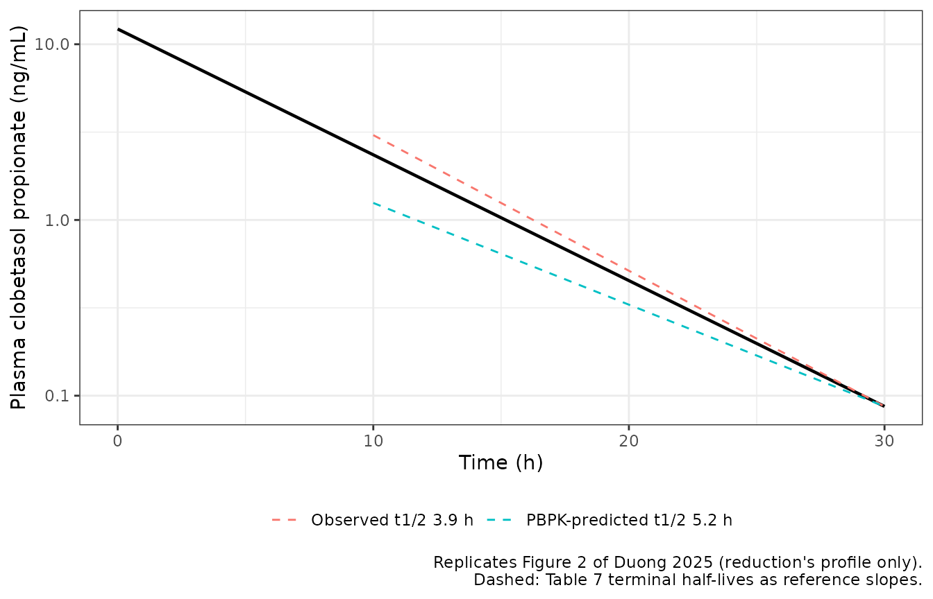
The reduction starts at dose / Vss (12.2 ng/mL). In
Figure 2 the platform’s mean profile falls from about 100 ng/mL to
roughly 15 ng/mL within the first half hour. That is the rapid
distribution phase into a small initial volume, which a single-volume
model omits. Between about 1 h and 20 h the reduction stays close to the
platform’s mean. Read approximately off Figure 2, the platform’s mean is
about 1.8 ng/mL at 10 h (reduction 2.4) and about 0.45 ng/mL at 20 h
(reduction 0.45). After that, the reduction’s shorter half-life carries
it below the platform’s mean: about 0.09 against 0.14 ng/mL at 30 h, at
the low edge of the observed values. Its terminal half-life (4.2 h) lies
between the platform’s 5.2 h and the observed 3.9 h.
PKNCA validation
conc <- sim |>
  dplyr::filter(!is.na(Cc)) |>
  dplyr::select(id, time, Cc, arm)

dose_df <- events |>
  dplyr::filter(evid == 1L) |>
  dplyr::select(id, time, amt, arm)

stopifnot(nrow(conc) > 0, nrow(dose_df) == 1L, any(conc$time == 0))

conc_obj <- PKNCA::PKNCAconc(conc, Cc ~ time | arm + id,
                             concu = "ng/mL", timeu = "h")
dose_obj <- PKNCA::PKNCAdose(dose_df, amt ~ time | arm + id,
                             doseu = "mg", route = "intravascular")

intervals <- data.frame(
  start = c(0, 0),
  end = c(30, Inf),
  auclast = c(TRUE, FALSE),
  aucinf.obs = c(FALSE, TRUE),
  half.life = c(FALSE, TRUE)
)

nca <- PKNCA::pk.nca(PKNCA::PKNCAdata(conc_obj, dose_obj,
                                      intervals = intervals))

nca_df <- as.data.frame(nca) |>
  dplyr::filter(PPTESTCD %in% c("auclast", "aucinf.obs", "half.life"))

knitr::kable(
  nca_df |>
    dplyr::mutate(PPORRES = signif(PPORRES, 4)) |>
    dplyr::select(arm, start, end, PPTESTCD, PPORRES, PPORRESU),
  caption = "PKNCA results for the simulated 2 mg intravenous dose."
)| arm | start | end | PPTESTCD | PPORRES | PPORRESU |
|---|---|---|---|---|---|
| Study A: 2 mg IV bolus | 0 | 30 | auclast | 73.550 | h*ng/mL |
| Study A: 2 mg IV bolus | 0 | Inf | half.life | 4.205 | h |
| Study A: 2 mg IV bolus | 0 | Inf | aucinf.obs | 74.070 | h*ng/mL |
Closed-form gates
For a one-compartment model after an intravenous bolus,
AUCinf = dose / CL and the terminal half-life is
log(2) * vc / cl, both exactly. These identities check the
NCA setup as much as the model.
get_nca <- function(p) {
  v <- nca_df$PPORRES[nca_df$PPTESTCD == p]
  if (length(v) != 1L) stop("no unique NCA row for ", p)
  v
}

vc_mod <- exp(theta[["lvc"]])
cl_mod <- exp(theta[["lcl_renal"]]) + exp(theta[["lcl_nonren"]])

gate <- tibble::tibble(
  Quantity = c("AUC0-inf (ng*h/mL)", "AUC0-30h (ng*h/mL)", "t1/2 (h)"),
  NCA = c(get_nca("aucinf.obs"), get_nca("auclast"), get_nca("half.life")),
  Closed_form = c(2 / cl_mod * 1000,
                  2 / cl_mod * 1000 * (1 - exp(-cl_mod / vc_mod * 30)),
                  log(2) * vc_mod / cl_mod)
) |>
  dplyr::mutate(pct = 100 * (NCA / Closed_form - 1))

knitr::kable(
  gate |>
    dplyr::mutate(dplyr::across(where(is.numeric), \(x) signif(x, 5))) |>
    dplyr::rename("Closed form" = Closed_form, "% diff" = pct),
  caption = "NCA output vs. the closed-form one-compartment identities."
)| Quantity | NCA | Closed form | % diff |
|---|---|---|---|
| AUC0-inf (ng*h/mL) | 74.0740 | 74.0740 | 0 |
| AUC0-30h (ng*h/mL) | 73.5470 | 73.5470 | 0 |
| t1/2 (h) | 4.2051 | 4.2051 | 0 |
# All three are exact for this model; what remains is trapezoidal error on
# the 0.05 h grid and ODE integration error. The bound sits well above the
# achieved agreement but far below any parameter-level mistake (a wrong
# volume or clearance moves these by tens of percent).
stopifnot(max(abs(gate$pct)) < 0.5)
Comparison against the published NCA
Against the paper’s own PBPK predictions
This comparison decides whether the reduction is faithful to the platform model. Table 7 reports the PBPK model’s predicted half-life and AUC for Study A. Its clearance row (26.2 L/h predicted, 27.6 L/h observed) is not tabulated separately: after an intravenous dose, clearance is dose / AUC0-inf, which the AUC0-inf row already tests. Nothing was tuned to reach these values.
nca_cmp <- nca_df |>
  dplyr::select(arm, PPTESTCD, PPORRES)

published_pred <- tibble::tribble(
  ~arm,     ~auclast, ~aucinf.obs, ~half.life,
  arm_lab,  78.2,     80.1,        5.2
)

cmp_pred <- nlmixr2lib::ncaComparisonTable(
  simulated = nca_cmp,
  reference = published_pred,
  by        = "arm",
  units     = c(auclast = "ng*h/mL", aucinf.obs = "ng*h/mL",
                half.life = "h"),
  tolerance_pct = 20
)

knitr::kable(
  cmp_pred,
  caption = paste("Reduction vs. the Simcyp predictions in Duong 2025",
                  "Table 7 (Study A, 2 mg IV; AUC0-30h in the auclast row).",
                  "* differs by >20%."),
  align = c("l", "l", "r", "r", "r")
)| NCA parameter | arm | Reference | Simulated | % diff |
|---|---|---|---|---|
| AUC0-∞ (obs) (ng*h/mL) | Study A: 2 mg IV bolus | 80.1 | 74.1 | -7.5% |
| AUClast (ng*h/mL) | Study A: 2 mg IV bolus | 78.2 | 73.5 | -6.0% |
| t½ (h) | Study A: 2 mg IV bolus | 5.2 | 4.21 | -19.1% |
# `% diff` is formatted as text (a trailing "*" marks rows over tolerance),
# so strip the formatting before testing. The solve is deterministic, so
# these bounds do not have to absorb any cohort sampling noise.
pct_pred <- suppressWarnings(
  as.numeric(gsub("[^0-9.eE+-]", "", as.character(cmp_pred[["% diff"]])))
)
stopifnot(sum(is.finite(pct_pred)) == 3L,
          max(abs(pct_pred), na.rm = TRUE) < 20)
cat(sprintf(paste("All %d comparisons against the PBPK predictions agree",
                  "within 20%%; largest discrepancy %.1f%%.\n"),
            sum(is.finite(pct_pred)), max(abs(pct_pred), na.rm = TRUE)))
#> All 3 comparisons against the PBPK predictions agree within 20%; largest discrepancy 19.1%.
How to read the table:
- AUC runs low by 6-8%. The platform’s simulated clearance runs slightly below its own 27 L/h input: the predicted AUC0-inf implies 2 mg / 80.1 ng*h/mL = 25.0 L/h. The reduction uses the 27 L/h that Table 6 gives as the model input and does not adopt the platform’s simulated output. Because the dose is flat (no body-weight dependence), the ratio 25.0 / 27 = 0.925 accounts for the whole AUC0-inf gap. The platform’s reported mean clearance of 26.2 L/h is a mean of individual clearances, which sits above dose divided by mean AUC.
-
The half-life is 19% short of the platform’s. This
is the cost of the mono-exponential reduction. The platform’s terminal
phase reflects slow return from peripheral tissues, while the
reduction’s single volume gives
log(2) * 163.8 / 27 = 4.2 h. The observed Study A half-life (3.9 h) sits closer to the reduction than to the platform.
Against the observed data
Table 7 also reports the observed Study A values (mean, with standard error). They are shown for completeness; they test the platform model as much as the reduction.
published_obs <- tibble::tribble(
  ~arm,     ~auclast, ~aucinf.obs, ~half.life,
  arm_lab,  73.3,     74.8,        3.9
)

cmp_obs <- nlmixr2lib::ncaComparisonTable(
  simulated = nca_cmp,
  reference = published_obs,
  by        = "arm",
  units     = c(auclast = "ng*h/mL", aucinf.obs = "ng*h/mL",
                half.life = "h"),
  tolerance_pct = 20
)

knitr::kable(
  cmp_obs,
  caption = paste("Reduction vs. observed Study A values in Duong 2025",
                  "Table 7. * differs by >20%."),
  align = c("l", "l", "r", "r", "r")
)| NCA parameter | arm | Reference | Simulated | % diff |
|---|---|---|---|---|
| AUC0-∞ (obs) (ng*h/mL) | Study A: 2 mg IV bolus | 74.8 | 74.1 | -1.0% |
| AUClast (ng*h/mL) | Study A: 2 mg IV bolus | 73.3 | 73.5 | +0.3% |
| t½ (h) | Study A: 2 mg IV bolus | 3.9 | 4.21 | +7.8% |
pct_obs <- suppressWarnings(
  as.numeric(gsub("[^0-9.eE+-]", "", as.character(cmp_obs[["% diff"]])))
)
stopifnot(sum(is.finite(pct_obs)) == 3L,
          max(abs(pct_obs), na.rm = TRUE) < 10)
The paper’s acceptance criterion is a predicted/observed ratio between 0.5 and 2.0. The reduction is within 10% of every observed Study A value.
Assumptions and deviations
-
Body weight of 70 kg is assumed. Table 6 states the
volume in L/kg, and no body weight for Study A appears in the paper or
its supplement. The 70 kg reference is the standing rounded standard,
and the paper corroborates it: the
Kpscalar was optimised to match the observed Study A volume of 164 L, and 164 / 2.34 = 70.1 kg.WTis recorded incovariatesDataExcludedrather than carried as a live covariate. The clearance is an absolute 27 L/h, so scaling volume alone would make the model internally inconsistent. -
Only the intravenous arm is reproduced. The topical
cream and ointment arms, the occlusion scenario, the atopic-dermatitis
skin-barrier-impairment model, the stratum-corneum concentrations and
the area-by-skin-condition simulations (Tables 7-9, Figures 3-6) all run
through Simcyp’s MechDermA model, whose equations and per-site skin
physiology the paper does not print. The oral arm is not reduced for the
two reasons shown above (unprinted
Fg * Fhand a Tmax that a single volume cannot reproduce). -
The reduction is mono-exponential. The source is a
full-PBPK model and only a lumped
Vssis reported, so no distribution phase can be reconstructed. The original Study A analysis reported an initial volume of about 18 L, but no inter-compartmental clearance, and it is a two-compartment fit of the data rather than the PBPK model. The cost is a missing early spike (first half hour) and a terminal half-life 19% shorter than the platform’s. - The clearance is the input, not the platform’s output. Table 6 gives 27 L/h as the in vivo clearance input. The Methods describe the Study A mean of 27.6 L/h as the initial estimate, and the Discussion repeats 27.6 L/h, but the final parameter table and the abstract both give 27 L/h, which is used here. The platform’s simulated clearance (26.2 L/h mean, 25.0 L/h from dose/AUC) is not adopted, since that would be tuning toward the answer key.
-
Two misprints in the source were resolved from the paper
itself.
- The Methods (“Intravenous administration”) give the Study A renal clearance as “2 L/h”. Table 6, Table 7 (observed 0.12, predicted 0.11 L/h) and the abstract all give 0.12 L/h, which is used.
- Table 7 lists the Study A intravenous dose as “0.02” g. Table 1 states 2 mg, and the observed AUC0-inf (74.8 ng*h/mL) times the observed clearance (27.6 L/h) gives 2.06 mg, so 2 mg is used.
- The intravenous dose is given as a bolus. Table 1 does not state an infusion duration, and Figure 2’s simulated profile starts at its peak at time zero.
-
No inter-individual variability and no residual
error. Duong 2025 is a PBPK simulation study, not a
population-PK fit. Its 5th-95th percentile bands are the spread of a
Simcyp virtual population driven by unpublished population files, not
estimated variance components. Rather than invent variances, the model
has no etas and
propSdis fixed at zero, so it is a deterministic typical-value simulator. -
Elimination is split only into renal and non-renal
arms. Table 6 prints CP’s elimination as an in vivo clearance
with a renal component, and no enzyme-level split. The renal arm is
carried as
lcl_renalbecause the paper prints it as a clearance; it does not change the plasma profile. - No errata were found. A EuropePMC search on 2026-11-10 found no correction notice for doi:10.1002/bcp.70102.