Pegcetacoplan geographic atrophy lesion area (Crass 2025)
Source:vignettes/articles/Crass_2025_pegcetacoplan_geographic_atrophy.Rmd
Crass_2025_pegcetacoplan_geographic_atrophy.RmdModel and source
Crass 2025 built three nested-in-purpose models of geographic atrophy (GA) lesion area, each reported with its own parameter table, so this paper contributes three model files:
mods <- c(
  progression       = "Crass_2025_pegcetacoplan_ga_progression",
  dose_response     = "Crass_2025_pegcetacoplan_ga_doseresponse",
  exposure_response = "Crass_2025_pegcetacoplan_ga_exposureresponse"
)
uis <- lapply(mods, function(nm) rxode2::rxode(readModelDb(nm)))
#> Warning: some etas defaulted to non-mu referenced, possible parsing error: etalrbase_study, etalslope_study, etalrbase_fellow, etalslope_fellow
#> as a work-around try putting the mu-referenced expression on a simple line
#> Warning: some etas defaulted to non-mu referenced, possible parsing error: etalrbase_study, etalslope_study, etalrbase_fellow, etalslope_fellow
#> as a work-around try putting the mu-referenced expression on a simple line
#> Warning: some etas defaulted to non-mu referenced, possible parsing error: etalrbase_study, etalslope_study, etalrbase_fellow, etalslope_fellow
#> as a work-around try putting the mu-referenced expression on a simple line| File | Role | Source table |
|---|---|---|
Crass_2025_pegcetacoplan_ga_progression |
Untreated natural-history layer, fit to sham-treated study eyes and untreated fellow eyes | Data S1 Table S4 |
Crass_2025_pegcetacoplan_ga_doseresponse |
Adds a per-regimen step-function pegcetacoplan effect on the study-eye growth rate | Data S1 Table S5 |
Crass_2025_pegcetacoplan_ga_exposureresponse |
Final PK/PD model; the drug effect is linear in log vitreous pegcetacoplan concentration | Data S1 Table S6 |
- Citation: Crass RL, Prem K, Gaudreault F, Lusk E, Ribeiro R, Chapel S, Baumal CR. Pharmacokinetic/pharmacodynamic analysis of geographic atrophy lesion area in patients receiving pegcetacoplan treatment or sham. CPT Pharmacometrics Syst Pharmacol. 2025;14(2):257-267. doi:10.1002/psp4.13264. Parameter values from Supporting Information Data S1, Table S6; model equations from Data S1 ‘The following equations describe the exposure-response model’. Vitreous concentrations were generated in the source analysis by an external population PK model reported only as a conference presentation (Crass RL, Smith B, Epling D, Chapel S, Prem K, Gaudreault F. Population pharmacokinetics of pegcetacoplan in patients with neovascular age-related macular degeneration and geographic atrophy. American Conference on Pharmacometrics, November 5-8 2023, National Harbor MD), which is not reproduced here; supply the concentration trajectory through the CEFFECT covariate column.
- Article: https://doi.org/10.1002/psp4.13264
- Supplement (Data S1, Tables S1-S6 and the model equations): https://doi.org/10.1002/psp4.13264 (Supporting Information)
All three share the same structural skeleton. Lesion area in each eye is algebraic in study time, not an integrated ODE:
Study eye and fellow eye are fit jointly with a 4x4 correlated
between-subject random-effect block over (initial area, slope) x (study
eye, fellow eye); every eta is Box-Cox transformed. Because there are no
d/dt() states, simulation event tables tag observation rows
with dvid (1 = study eye, 2 = fellow eye) and leave
cmt missing.
Population
The analysis pooled 1501 patients with GA secondary to age-related macular degeneration from three trials: the 12-month phase II FILLY trial (NCT02503332, n = 246) and the 24-month phase III OAKS (NCT03525613, n = 636) and DERBY (NCT03525600, n = 620) trials. Patients were randomised 2:2:1:1 to intravitreal pegcetacoplan 15 mg monthly (n = 505), pegcetacoplan 15 mg every other month (n = 498), sham monthly, or sham every other month (n = 498 combined sham).
The population was elderly (median age 79 years, range 60-100), predominantly female (62%) and White (94%). At baseline 81% had bilateral GA, 63% had subfoveal lesions, 70% had multifocal lesions, and 45% had more than 20 intermediate or large drusen groups in the study eye. Median baseline lesion area was 8 mm^2 (range 2-18); trial entry required a total GA lesion area between 2.5 and 17.5 mm^2 with at least one lesion >= 1.25 mm^2 if multifocal. These figures are Table 1 of Crass 2025. Note that Table 1 reports n = 1502 including one patient without quantifiable PK samples who was excluded from the PK/PD modelling analyses.
The same information is available programmatically:
str(uis$exposure_response$population, max.level = 1, give.attr = FALSE)
#> List of 13
#>  $ species       : chr "human"
#>  $ n_subjects    : int 1501
#>  $ n_studies     : int 3
#>  $ age_range     : chr "60-100 years (pooled); FILLY enrolled patients aged >= 50 years, OAKS and DERBY >= 60 years"
#>  $ age_median    : chr "79 years"
#>  $ weight_range  : chr NA
#>  $ weight_median : chr NA
#>  $ sex_female_pct: num 62
#>  $ race_ethnicity: Named num [1:5] 94 0.4 0.5 0.2 5
#>  $ disease_state : chr "Geographic atrophy secondary to age-related macular degeneration. Baseline total GA lesion area 2.5-17.5 mm^2 i"| __truncated__
#>  $ dose_range    : chr "Intravitreal pegcetacoplan 15 mg (0.1 mL of 150 mg/mL) monthly (n = 505) or every other month (n = 498), or sha"| __truncated__
#>  $ regions       : chr "(not reported in Crass 2025)"
#>  $ notes         : chr "Pooled from the 12-month phase II FILLY trial (NCT02503332, n = 246) and the 24-month phase III OAKS (NCT035256"| __truncated__
Source trace
Every ini() entry in each model file carries an in-file
comment naming its source location. Collected here for review:
| Parameter | Progression (Table S4) | Dose-response (Table S5) | PK/PD (Table S6) |
|---|---|---|---|
| Study eye initial lesion area, mm^2 | 7.73 | 7.69 | 7.69 |
| Study eye time slope, mm^2/day | 0.00554 | 0.00565 | 0.00559 |
| Fellow eye initial lesion area, mm^2 | 7.28 | 7.25 | 7.25 |
| Fellow eye time slope, mm^2/day | 0.00486 | 0.00491 | 0.00490 |
| Unilateral GA on study eye initial area | -0.169 | -0.124 | -0.123 |
| Unilateral GA on study eye slope | -0.151 | -0.138 | -0.139 |
| No subfoveal involvement on slope | 0.179 | 0.119 | 0.118 |
| Unifocal GA on slope | -0.156 | -0.165 | -0.164 |
| More (>20) drusen groups on slope | -0.147 | -0.132 | -0.130 |
| Monthly drug effect, proportion | – | -0.204 | – |
| Every-other-month drug effect, proportion | – | -0.172 | – |
| Drug effect slope, proportion/log(ug/mL) | – | – | -0.026 |
| Box-Cox lambda, study initial / study slope | -0.306 / -0.270 | -0.312 / -0.281 | -0.313 / -0.287 |
| Box-Cox lambda, fellow initial / fellow slope | -0.540 / -0.348 | -0.536 / -0.404 | -0.537 / -0.405 |
| Residual, study eye proportional / additive (mm^2) | 0.0244 / 0.192 | 0.0276 / 0.175 | 0.0276 / 0.175 |
| Residual, fellow eye proportional / additive (mm^2) | 0.0310 / 0.207 | 0.0309 / 0.207 | 0.0309 / 0.207 |
| IIV 4x4 block (variances, covariances) | Table S4 | Table S5 | Table S6 |
Model equations are transcribed from the Data S1 block headed “The
following equations describe the exposure-response model”, which defines
INIT_i,study, SLOPE_i,study,
DSLOPE_i,study(t), INIT_i,fellow and
SLOPE_i,fellow and names each theta.
Interindividual-variability block
The encoded 4x4 blocks are checked here directly against the correlations the paper reports in the transformed column of Tables S4-S6 (and, for the study-vs-fellow slope pair, against the value quoted in the Discussion).
omega_corr <- function(ui) {
  om <- ui$omega
  cv <- stats::cov2cor(om)
  data.frame(
    pair = c("slope study : init study", "init fellow : init study",
             "init fellow : slope study", "slope fellow : init study",
             "slope fellow : slope study", "slope fellow : init fellow"),
    encoded = c(cv[2, 1], cv[3, 1], cv[3, 2], cv[4, 1], cv[4, 2], cv[4, 3])
  )
}

corr_tab <- omega_corr(uis$progression) |>
  dplyr::rename("Random-effect pair" = pair, "Encoded (Table S4)" = encoded) |>
  dplyr::mutate(
    `Published rho` = c(0.411, 0.676, 0.351, 0.445, 0.705, 0.408),
    `Abs. difference` = abs(`Encoded (Table S4)` - `Published rho`)
  )

knitr::kable(
  corr_tab, digits = 4,
  caption = paste(
    "Correlations implied by the encoded Table S4 covariance block vs the",
    "values printed in the source table. The 0.705 study-vs-fellow slope",
    "correlation is the value quoted in the Crass 2025 Discussion."
  )
)| Random-effect pair | Encoded (Table S4) | Published rho | Abs. difference |
|---|---|---|---|
| slope study : init study | 0.4109 | 0.411 | 1e-04 |
| init fellow : init study | 0.6769 | 0.676 | 9e-04 |
| init fellow : slope study | 0.3513 | 0.351 | 3e-04 |
| slope fellow : init study | 0.4440 | 0.445 | 1e-03 |
| slope fellow : slope study | 0.7043 | 0.705 | 7e-04 |
| slope fellow : init fellow | 0.4083 | 0.408 | 3e-04 |
Every encoded correlation reproduces the published value to within 0.002, so the covariance block was transcribed correctly (the residual difference is the source table’s three-significant-figure rounding).
Virtual cohort
Original patient-level data are not publicly available. The simulations below use virtual cohorts whose baseline-disease covariate distributions match the published Table 1 marginals. Cohort size is 200 per arm.
set.seed(20250213)

VISIT_DAYS <- round(seq(0, 24, by = 1) * 30.4375, 3)  # monthly visits to month 24

# Build one arm as an event table. Both endpoints are algebraic, so
# observation rows carry dvid (1 = study eye, 2 = fellow eye) and a missing
# cmt; there are no dosing records at all -- the pegcetacoplan regimen enters
# through REGI_QM / REGI_Q2M (dose-response) or CEFFECT (exposure-response).
make_arm <- function(n, arm, id_offset = 0L,
                     regi_qm = 0, regi_q2m = 0, ceffect = 0,
                     unilateral = NULL, nonsubfoveal = NULL,
                     unifocal = NULL, drusen = NULL,
                     dvids = c(1L, 2L)) {
  subj <- tibble::tibble(
    id                  = id_offset + seq_len(n),
    arm                 = arm,
    REGI_QM             = regi_qm,
    REGI_Q2M            = regi_q2m,
    CEFFECT             = ceffect,
    DIS_GA_UNILATERAL   = if (is.null(unilateral))   stats::rbinom(n, 1, 0.19) else unilateral,
    DIS_GA_NONSUBFOVEAL = if (is.null(nonsubfoveal)) stats::rbinom(n, 1, 0.37) else nonsubfoveal,
    DIS_GA_UNIFOCAL     = if (is.null(unifocal))     stats::rbinom(n, 1, 0.30) else unifocal,
    DRUSEN_GT20         = if (is.null(drusen))       stats::rbinom(n, 1, 0.45) else drusen
  )
  subj |>
    tidyr::crossing(time = VISIT_DAYS, dvid = dvids) |>
    dplyr::mutate(evid = 0L, amt = NA_real_, cmt = NA_integer_) |>
    dplyr::arrange(id, dvid, time)
}

KEEP_COLS <- c("arm", "REGI_QM", "REGI_Q2M", "CEFFECT", "DIS_GA_UNILATERAL",
               "DIS_GA_NONSUBFOVEAL", "DIS_GA_UNIFOCAL", "DRUSEN_GT20")

# Deterministic (typical-value) solve. `omega = NA` suppresses the random
# effects so the prediction is the typical individual rather than a population
# median; it is used in preference to zeroRe() because zeroRe() mutates the ui
# it is handed, and the same ui objects are reused across chunks here.
solve_typical <- function(ui, events) {
  rxode2::rxSolve(ui, events = events, omega = NA, keep = KEEP_COLS,
                  returnType = "data.frame")
}
Untreated disease progression (paper Results, “Disease progression model”)
Crass 2025 reports that lesion growth in untreated eyes “was estimated at 2.02 mm^2/year from an estimated baseline lesion area of 7.73 mm^2 in patients with bilateral GA, subfoveal involvement, multifocal distribution, and fewer (<= 20) intermediate or large drusen groups” – i.e. the reference covariate state in which every indicator is 0.
ref_arm <- make_arm(
  n = 1L, arm = "reference (all covariates 0)", dvids = 1L,
  unilateral = 0, nonsubfoveal = 0, unifocal = 0, drusen = 0
)

nh <- solve_typical(uis$progression, ref_arm)

nh_summary <- nh |>
  dplyr::summarise(
    `Study eye baseline (mm^2)`        = dplyr::first(rbaseStudy),
    `Study eye growth (mm^2/year)`     = dplyr::first(slopeStudy) * 365.25,
    `Fellow eye baseline (mm^2)`       = dplyr::first(rbaseFellow),
    `Fellow eye growth (mm^2/year)`    = dplyr::first(slopeFellow) * 365.25
  ) |>
  tidyr::pivot_longer(dplyr::everything(), names_to = "Quantity", values_to = "Simulated")

nh_summary$Published <- c(7.73, 2.02, 7.28, NA_real_)

knitr::kable(
  nh_summary, digits = 3,
  caption = paste(
    "Typical untreated GA progression from the disease-progression model",
    "(Table S4) vs the values stated in the Crass 2025 Results. The fellow-eye",
    "annual rate is not quoted numerically in the paper."
  )
)| Quantity | Simulated | Published |
|---|---|---|
| Study eye baseline (mm^2) | 7.730 | 7.73 |
| Study eye growth (mm^2/year) | 2.023 | 2.02 |
| Fellow eye baseline (mm^2) | 7.280 | 7.28 |
| Fellow eye growth (mm^2/year) | 1.775 | NA |
stopifnot(
  abs(nh_summary$Simulated[1] - 7.73) < 0.005,
  abs(nh_summary$Simulated[2] - 2.02) < 0.01,
  abs(nh_summary$Simulated[3] - 7.28) < 0.005
)
The model reproduces both headline numbers exactly: 2.023 mm^2/year of study-eye lesion growth from a 7.73 mm^2 baseline.
nh_long <- nh |>
  dplyr::select(time, lesionStudy, lesionFellow) |>
  dplyr::distinct() |>
  tidyr::pivot_longer(c(lesionStudy, lesionFellow),
                      names_to = "Eye", values_to = "area") |>
  dplyr::mutate(Eye = ifelse(Eye == "lesionStudy", "Study eye", "Fellow eye"),
                month = time / 30.4375)

ggplot(nh_long, aes(month, area, colour = Eye)) +
  geom_line(linewidth = 1) +
  scale_x_continuous(breaks = seq(0, 24, 6)) +
  labs(x = "Study month", y = expression(GA~lesion~area~(mm^2)),
       colour = NULL,
       title = "Typical untreated GA lesion-area progression",
       caption = paste("Reference covariate state (bilateral, subfoveal,",
                       "multifocal, <= 20 drusen groups). Disease-progression",
                       "model, Crass 2025 Table S4.")) +
  theme_minimal()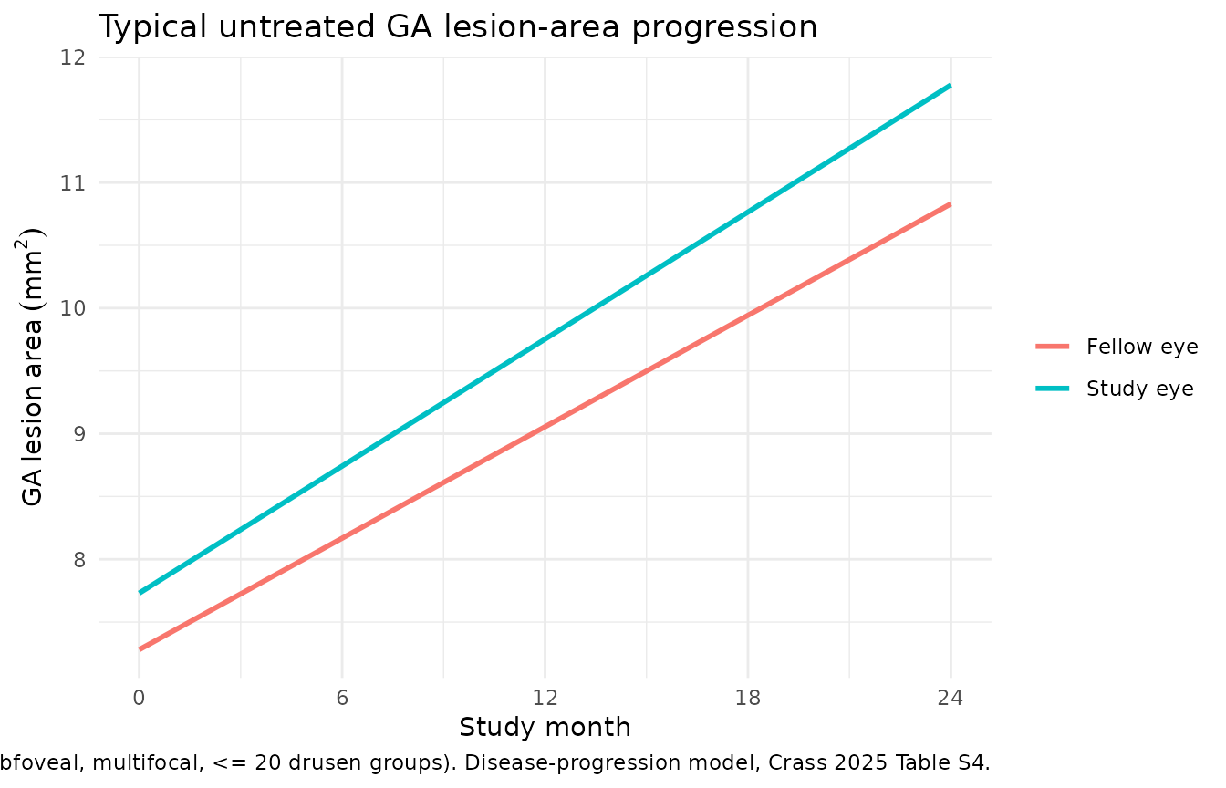
Baseline-disease covariate effects (replicates Figure 2)
Figure 2 of Crass 2025 is a forest plot of the fold-change in
predicted median lesion-area growth at month 24 for each
baseline-disease covariate. Because every covariate enters the study-eye
slope as a proportional shift (1 + theta * indicator) and
growth from baseline is slope * t, the fold-effect is
exactly 1 + theta. The check below computes it by
simulation rather than asserting the algebra.
cov_specs <- tibble::tribble(
  ~label,                              ~covariate,
  "Unilateral vs bilateral GA",        "DIS_GA_UNILATERAL",
  "Nonsubfoveal vs subfoveal",         "DIS_GA_NONSUBFOVEAL",
  "Unifocal vs multifocal",            "DIS_GA_UNIFOCAL",
  "> 20 vs <= 20 drusen groups",       "DRUSEN_GT20"
)

# Growth from baseline at month 24 for a typical individual with one
# covariate switched on, relative to the all-zero reference state.
growth_24mo <- function(ui, covariate, value) {
  args <- list(n = 1L, arm = "x", dvids = 1L,
               unilateral = 0, nonsubfoveal = 0, unifocal = 0, drusen = 0)
  slot <- c(DIS_GA_UNILATERAL = "unilateral", DIS_GA_NONSUBFOVEAL = "nonsubfoveal",
            DIS_GA_UNIFOCAL = "unifocal", DRUSEN_GT20 = "drusen")[[covariate]]
  args[[slot]] <- value
  s <- solve_typical(ui, do.call(make_arm, args))
  end <- s$lesionStudy[which.max(s$time)]
  start <- s$lesionStudy[which.min(s$time)]
  end - start
}

fig2 <- cov_specs |>
  dplyr::rowwise() |>
  dplyr::mutate(
    Simulated = growth_24mo(uis$exposure_response, covariate, 1) /
      growth_24mo(uis$exposure_response, covariate, 0)
  ) |>
  dplyr::ungroup()

fig2$Published <- c(0.860, 1.12, 0.837, 0.869)
fig2$`Published 90% CI` <- c("0.808, 0.913", "1.07, 1.16",
                             "0.800, 0.872", "0.837, 0.904")
fig2$`Abs. difference` <- abs(fig2$Simulated - fig2$Published)

fig2 |>
  dplyr::select(-covariate) |>
  dplyr::rename("Baseline disease factor" = label,
                "Simulated fold-change" = Simulated,
                "Published fold-change" = Published) |>
  knitr::kable(
    digits = 3,
    caption = paste(
      "Fold-change in month-24 study-eye lesion growth per baseline disease",
      "factor. Replicates Figure 2 of Crass 2025; published point estimates",
      "are quoted in the Results section."
    )
)| Baseline disease factor | Simulated fold-change | Published fold-change | Published 90% CI | Abs. difference |
|---|---|---|---|---|
| Unilateral vs bilateral GA | 0.861 | 0.860 | 0.808, 0.913 | 0.001 |
| Nonsubfoveal vs subfoveal | 1.118 | 1.120 | 1.07, 1.16 | 0.002 |
| Unifocal vs multifocal | 0.836 | 0.837 | 0.800, 0.872 | 0.001 |
| > 20 vs <= 20 drusen groups | 0.870 | 0.869 | 0.837, 0.904 | 0.001 |
All four fold-effects reproduce the published values to within
0.0020. The small residuals are the paper’s rounding of
1 + theta to three significant figures.
Note that these are the final PK/PD model coefficients
(Table S6). The disease-progression model (Table S4) fits somewhat
larger baseline-disease effects – for instance
1 + 0.179 = 1.179 rather than 1.12 for nonsubfoveal
involvement – because it was fit to untreated eyes only. The paper’s
Figure 2 values match Table S6.
Dose-response treatment effect (replicates Figure 3)
The dose-response model estimates one step-function drug effect per active regimen. Crass 2025 reports a “0.80-fold lower (95% CI: 0.75, 0.84)” rate of disease progression on pegcetacoplan monthly and “0.83-fold lower (95% CI: 0.78, 0.87)” on every other month, equivalent to point estimates of 20.4% and 17.2% reductions in lesion-area change from baseline.
dr_arms <- dplyr::bind_rows(
  make_arm(1L, "Sham",                     id_offset =  0L, dvids = 1L,
           unilateral = 0, nonsubfoveal = 0, unifocal = 0, drusen = 0),
  make_arm(1L, "Pegcetacoplan monthly",    id_offset = 10L, regi_qm  = 1, dvids = 1L,
           unilateral = 0, nonsubfoveal = 0, unifocal = 0, drusen = 0),
  make_arm(1L, "Pegcetacoplan EOM",        id_offset = 20L, regi_q2m = 1, dvids = 1L,
           unilateral = 0, nonsubfoveal = 0, unifocal = 0, drusen = 0)
)

dr <- solve_typical(uis$dose_response, dr_arms)
#> Warning: multi-subject simulation without without 'omega'

dr_effect <- dr |>
  dplyr::group_by(arm) |>
  dplyr::summarise(
    growth24 = lesionStudy[which.max(time)] - lesionStudy[which.min(time)],
    .groups = "drop"
  ) |>
  dplyr::mutate(
    ratio_vs_sham = growth24 / growth24[arm == "Sham"],
    pct_reduction = 100 * (1 - ratio_vs_sham)
  ) |>
  dplyr::filter(arm != "Sham")

dr_effect$`Published ratio` <- c(0.83, 0.80)
dr_effect$`Published 95% CI` <- c("0.78, 0.87", "0.75, 0.84")
dr_effect$`Published % reduction` <- c(17.2, 20.4)

dr_effect |>
  dplyr::select(arm, growth24, ratio_vs_sham, `Published ratio`,
                `Published 95% CI`, pct_reduction, `Published % reduction`) |>
  dplyr::rename("Regimen" = arm,
                "Month-24 growth (mm^2)" = growth24,
                "Simulated ratio vs sham" = ratio_vs_sham,
                "Simulated % reduction" = pct_reduction) |>
  knitr::kable(
    digits = 3,
    caption = paste(
      "Pegcetacoplan effect on month-24 GA lesion growth relative to sham.",
      "Replicates Figure 3 of Crass 2025 (dose-response model, Table S5)."
    )
)| Regimen | Month-24 growth (mm^2) | Simulated ratio vs sham | Published ratio | Published 95% CI | Simulated % reduction | Published % reduction |
|---|---|---|---|---|---|---|
| Pegcetacoplan EOM | 3.417 | 0.828 | 0.83 | 0.78, 0.87 | 17.2 | 17.2 |
| Pegcetacoplan monthly | 3.285 | 0.796 | 0.80 | 0.75, 0.84 | 20.4 | 20.4 |
stopifnot(
  nrow(dr_effect) == 2L,
  all(abs(dr_effect$ratio_vs_sham - dr_effect$`Published ratio`) < 0.01),
  all(abs(dr_effect$pct_reduction - dr_effect$`Published % reduction`) < 0.1)
)
Both regimens reproduce the published effect sizes: the simulated ratios agree with the published 0.80 and 0.83 to within 0.01, and the percent reductions match the published 20.4% and 17.2% to the tenth of a percent.
Exposure-response relationship (replicates Figure 4)
The final PK/PD model replaces the step function with a term linear in the log of the instantaneous individual-predicted vitreous pegcetacoplan concentration:
The +1 inside the logarithm keeps the untreated state
well defined: at CEFFECT = 0 the term vanishes and the
treated slope collapses to the untreated slope. Figure 4 of Crass 2025
plots this curve with the dose-response point estimates overlaid as
horizontal reference lines. The chunk below reproduces the curve by
simulation and then back-solves the vitreous
concentration at which it crosses each dose-response line – the
quantitative form of the paper’s claim that “this PK/PD curve was
consistent with the point estimates for dose response within the
predicted range of exposures”.
conc_grid <- exp(seq(log(1), log(5000), length.out = 60))

er_arms <- dplyr::bind_rows(lapply(seq_along(conc_grid), function(i) {
  make_arm(1L, arm = sprintf("C%03d", i), id_offset = (i - 1L) * 10L, dvids = 1L,
           ceffect = conc_grid[i],
           unilateral = 0, nonsubfoveal = 0, unifocal = 0, drusen = 0)
}))

er <- solve_typical(uis$exposure_response, er_arms)
#> Warning: multi-subject simulation without without 'omega'

er_curve <- er |>
  dplyr::group_by(arm) |>
  dplyr::summarise(CEFFECT = dplyr::first(CEFFECT),
                   rel_rate = dplyr::first(dslopeStudy) / dplyr::first(slopeStudy),
                   .groups = "drop")

# Back-solve the vitreous concentration reproducing each dose-response point
# estimate: 1 + theta23 * log(C + 1) = ratio  =>  C = exp((ratio - 1)/theta23) - 1
theta23 <- -0.026
implied <- tibble::tibble(
  arm   = c("Pegcetacoplan EOM", "Pegcetacoplan monthly"),
  ratio = c(1 - 0.172, 1 - 0.204)
) |>
  dplyr::mutate(conc_ugmL = exp((ratio - 1) / theta23) - 1)

ggplot(er_curve, aes(CEFFECT, rel_rate)) +
  geom_line(linewidth = 1) +
  geom_hline(data = implied, aes(yintercept = ratio, colour = arm),
             linetype = "dashed") +
  geom_vline(data = implied, aes(xintercept = conc_ugmL, colour = arm),
             linetype = "dotted") +
  scale_x_log10() +
  labs(x = "Vitreous pegcetacoplan concentration (ug/mL, log scale)",
       y = "GA lesion growth rate relative to untreated",
       colour = "Dose-response estimate",
       title = "Exposure-response for GA lesion growth rate",
       caption = paste("Replicates Figure 4 of Crass 2025. Dashed lines are the",
                       "dose-response point estimates; dotted lines mark the",
                       "vitreous concentration at which the PK/PD curve",
                       "reproduces them.")) +
  theme_minimal()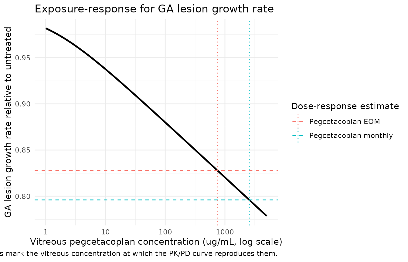
DOSE_MG        <- 15      # Crass 2025 Methods: intravitreal pegcetacoplan 15 mg
VITREOUS_ML    <- 4       # Crass 2025 Methods: "the volume of the vitreous compartment was set to 4 mL"
peak_conc_ugmL <- DOSE_MG * 1000 / VITREOUS_ML

implied_tab <- implied |>
  dplyr::mutate(
    pct_of_immediate_postdose = 100 * conc_ugmL / peak_conc_ugmL,
    `Published PK/PD ratio` = c(0.83, 0.80)
  ) |>
  dplyr::rename("Regimen" = arm,
                "Dose-response ratio" = ratio,
                "Implied vitreous conc. (ug/mL)" = conc_ugmL,
                "% of immediate post-dose conc." = pct_of_immediate_postdose)

knitr::kable(
  implied_tab, digits = c(0, 3, 0, 1, 2),
  caption = paste(
    "Vitreous pegcetacoplan concentration at which the exposure-response curve",
    "reproduces each dose-response point estimate, expressed as a percentage",
    "of the immediate post-dose concentration (15 mg into a 4 mL vitreous",
    "volume =", format(peak_conc_ugmL, big.mark = ","), "ug/mL). The published",
    "PK/PD predictions of treatment effect were 0.80 (90% CI 0.77, 0.84)",
    "monthly and 0.83 (90% CI 0.80, 0.86) every other month."
  )
)| Regimen | Dose-response ratio | Implied vitreous conc. (ug/mL) | % of immediate post-dose conc. | Published PK/PD ratio |
|---|---|---|---|---|
| Pegcetacoplan EOM | 0.828 | 745 | 19.9 | 0.83 |
| Pegcetacoplan monthly | 0.796 | 2555 | 68.1 | 0.80 |
stopifnot(
  # The curve must pass through both dose-response point estimates at
  # concentrations that are physically reachable, i.e. below the immediate
  # post-dose concentration of a 15 mg intravitreal injection.
  all(implied_tab$`Implied vitreous conc. (ug/mL)` < peak_conc_ugmL),
  all(implied_tab$`% of immediate post-dose conc.` > 1),
  # Monthly dosing must imply the higher sustained concentration.
  implied_tab$`Implied vitreous conc. (ug/mL)`[2] >
    implied_tab$`Implied vitreous conc. (ug/mL)`[1]
)
The two models are mutually consistent and physically coherent: reproducing the monthly dose-response effect requires a sustained vitreous concentration of about 2,555 ug/mL (68% of the concentration reached immediately after a 15 mg injection into a 4 mL vitreous volume), and the every-other-month effect about 745 ug/mL (20%). The 3.4-fold ratio between them is the expected direction and magnitude for halving the dosing frequency of a drug eliminated slowly from the vitreous, and both sit below the immediate post-dose concentration, as they must. This reproduces the paper’s own reconciliation of the two models without requiring the upstream population PK model, which was not available when this model was built (see Assumptions and deviations).
Evaluating the same relationship directly at the immediate post-dose concentration gives 0.786, which brackets the 0.80 monthly dose-response estimate from below – as expected, since the concentration decays between injections.
Population simulation with between-subject variability
A 200-subject-per-arm stochastic simulation of the dose-response model, sampling baseline-disease covariates from the Table 1 marginals. This reproduces the shape of the Figure S2 visual predictive checks.
set.seed(20250213)
N_PER_ARM <- 200L
VPC_SEED  <- 4242L

# One covariate draw, reused across all three arms. Pairing the arms on
# covariates AND on the random-effect draws (same seed before each solve, same
# id numbering within each arm) removes the between-arm imbalance that would
# otherwise swamp the 3-percentage-point difference between the monthly and
# every-other-month treatment effects.
cov_draw <- tibble::tibble(
  unilateral   = stats::rbinom(N_PER_ARM, 1, 0.19),
  nonsubfoveal = stats::rbinom(N_PER_ARM, 1, 0.37),
  unifocal     = stats::rbinom(N_PER_ARM, 1, 0.30),
  drusen       = stats::rbinom(N_PER_ARM, 1, 0.45)
)

solve_arm <- function(arm, regi_qm = 0, regi_q2m = 0) {
  ev <- make_arm(N_PER_ARM, arm, regi_qm = regi_qm, regi_q2m = regi_q2m,
                 unilateral   = cov_draw$unilateral,
                 nonsubfoveal = cov_draw$nonsubfoveal,
                 unifocal     = cov_draw$unifocal,
                 drusen       = cov_draw$drusen)
  stopifnot(!anyDuplicated(ev[, c("id", "time", "dvid")]))
  set.seed(VPC_SEED)   # identical eta draws in every arm -> paired comparison
  rxode2::rxSolve(uis$dose_response, events = ev, keep = KEEP_COLS,
                  returnType = "data.frame")
}

vpc <- dplyr::bind_rows(
  solve_arm("Sham"),
  solve_arm("Pegcetacoplan monthly", regi_qm  = 1),
  solve_arm("Pegcetacoplan EOM",     regi_q2m = 1)
)

stopifnot(
  nrow(vpc) > 0,
  length(unique(vpc$arm)) == 3L,
  !anyDuplicated(unique(vpc[, c("arm", "id", "time", "CMT")]))
)
vpc_bands <- vpc |>
  dplyr::filter(CMT == 1L) |>
  dplyr::mutate(month = time / 30.4375) |>
  dplyr::group_by(arm, month) |>
  dplyr::summarise(
    Q05 = stats::quantile(sim, 0.05),
    Q50 = stats::quantile(sim, 0.50),
    Q95 = stats::quantile(sim, 0.95),
    .groups = "drop"
  )

ggplot(vpc_bands, aes(month, Q50)) +
  geom_ribbon(aes(ymin = Q05, ymax = Q95), alpha = 0.25) +
  geom_line(linewidth = 0.9) +
  facet_wrap(~arm) +
  scale_x_continuous(breaks = seq(0, 24, 6)) +
  labs(x = "Study month", y = expression(Study~eye~GA~lesion~area~(mm^2)),
       title = "Simulated study-eye GA lesion area by treatment arm",
       caption = paste("Median and 5th-95th percentile of the simulated",
                       "observation (200 subjects per arm). Reproduces the",
                       "shape of Figure S2 of Crass 2025.")) +
  theme_minimal()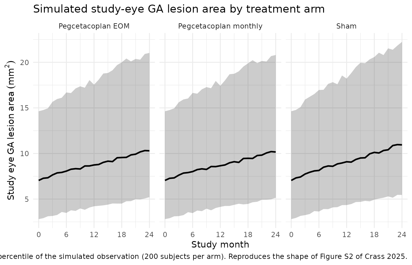
fellow_bands <- vpc |>
  dplyr::filter(CMT == 2L, arm == "Sham") |>
  dplyr::mutate(month = time / 30.4375) |>
  dplyr::group_by(month) |>
  dplyr::summarise(
    Q05 = stats::quantile(sim, 0.05),
    Q50 = stats::quantile(sim, 0.50),
    Q95 = stats::quantile(sim, 0.95),
    .groups = "drop"
  )

ggplot(fellow_bands, aes(month, Q50)) +
  geom_ribbon(aes(ymin = Q05, ymax = Q95), alpha = 0.25) +
  geom_line(linewidth = 0.9) +
  scale_x_continuous(breaks = seq(0, 24, 6)) +
  labs(x = "Study month", y = expression(Fellow~eye~GA~lesion~area~(mm^2)),
       title = "Simulated untreated fellow-eye GA lesion area",
       caption = paste("Median and 5th-95th percentile of the simulated",
                       "observation. The fellow eye is never treated, so this",
                       "panel is identical across arms by construction.")) +
  theme_minimal()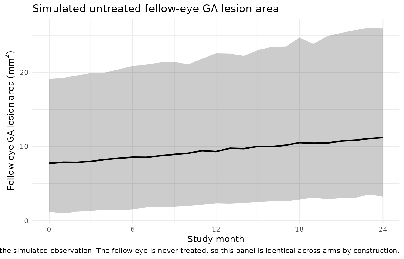
Because the three arms share covariate draws and random-effect draws, each simulated subject appears once per arm and can be compared with their own sham trajectory. The drug effect is a pure multiplicative shift on the study-eye slope, so this paired ratio must recover the typical-value ratio exactly – an unpaired between-arm comparison at this cohort size would be dominated by sampling noise, since the between-subject spread in growth rate is an order of magnitude larger than the 3-percentage-point difference between the monthly and every-other-month effects.
per_subject <- vpc |>
  dplyr::filter(CMT == 1L) |>
  dplyr::group_by(arm, id) |>
  dplyr::summarise(
    growth = lesionStudy[which.max(time)] - lesionStudy[which.min(time)],
    .groups = "drop"
  )

# Paired per-subject ratio vs the same subject's sham trajectory.
sham_growth <- per_subject |>
  dplyr::filter(arm == "Sham") |>
  dplyr::select(id, sham_growth = growth)

vpc_growth <- per_subject |>
  dplyr::left_join(sham_growth, by = "id") |>
  dplyr::group_by(arm) |>
  dplyr::summarise(
    median_growth       = stats::median(growth),
    median_paired_ratio = stats::median(growth / sham_growth),
    .groups = "drop"
  )

vpc_growth$`Typical-value ratio` <- c(0.828, 0.796, 1.000)[
  match(vpc_growth$arm, c("Pegcetacoplan EOM", "Pegcetacoplan monthly", "Sham"))
]

vpc_growth |>
  dplyr::rename("Regimen" = arm,
                "Median month-24 growth (mm^2)" = median_growth,
                "Median paired ratio vs sham" = median_paired_ratio) |>
  knitr::kable(
    digits = 3,
    caption = paste(
      "Population month-24 study-eye lesion growth from the 200-per-arm",
      "stochastic simulation. The arms share covariate draws and random-effect",
      "draws, so each subject can be compared with their own sham trajectory.",
      "Because the drug effect is a pure multiplicative shift on the slope,",
      "the paired ratio must recover the typical-value ratio exactly."
    )
)| Regimen | Median month-24 growth (mm^2) | Median paired ratio vs sham | Typical-value ratio |
|---|---|---|---|
| Pegcetacoplan EOM | 3.077 | 0.828 | 0.828 |
| Pegcetacoplan monthly | 2.958 | 0.796 | 0.796 |
| Sham | 3.716 | 1.000 | 1.000 |
Dimensional and residual-error checks
ui_er <- uis$exposure_response
ini_er <- ui_er$iniDf
getval <- function(nm) {
  v <- ini_er$est[!is.na(ini_er$name) & ini_er$name == nm]
  if (length(v) != 1L) stop("no unique ini() entry named '", nm, "'")
  v
}

slope_day  <- exp(getval("lslope_study"))
rbase_mm2  <- exp(getval("lrbase_study"))
prop_study <- getval("propSd_lesionStudy")
add_study  <- getval("addSd_lesionStudy")

checks <- tibble::tribble(
  ~Check, ~Value, ~Expectation,
  "Study-eye slope (mm^2/day) x 365.25",
  slope_day * 365.25,
  "About 2 mm^2/year, the published untreated growth rate",

  "Month-24 growth as % of baseline area",
  100 * slope_day * 730.5 / rbase_mm2,
  "About 50% -- a 7.7 mm^2 lesion grows by about 4 mm^2 over 2 years",

  "Combined residual SD at a 10 mm^2 lesion (mm^2)",
  sqrt((prop_study * 10)^2 + add_study^2),
  "Under 0.5 mm^2, i.e. a few percent CV, consistent with planimetry on FAF",

  "Relative growth rate at CEFFECT = 0",
  1 + theta23 * log(0 + 1),
  "Exactly 1 -- the untreated state must be recovered"
)

knitr::kable(checks, digits = 3,
caption = "Dimensional and magnitude sanity checks.")| Check | Value | Expectation |
|---|---|---|
| Study-eye slope (mm^2/day) x 365.25 | 2.042 | About 2 mm^2/year, the published untreated growth rate |
| Month-24 growth as % of baseline area | 53.101 | About 50% – a 7.7 mm^2 lesion grows by about 4 mm^2 over 2 years |
| Combined residual SD at a 10 mm^2 lesion (mm^2) | 0.327 | Under 0.5 mm^2, i.e. a few percent CV, consistent with planimetry on FAF |
| Relative growth rate at CEFFECT = 0 | 1.000 | Exactly 1 – the untreated state must be recovered |
Assumptions and deviations
-
The upstream population PK model is not reproduced.
The vitreous pegcetacoplan concentration that drives the
exposure-response model was generated in the source analysis by a
separate population PK model reported only as a conference presentation
(Crass et al., American Conference on Pharmacometrics, November 2023),
which was not available when this model was built. That model is
therefore not encoded here:
Crass_2025_pegcetacoplan_ga_exposureresponseconsumes the vitreous concentration as theCEFFECTtime-varying covariate, exactly as the source NONMEM run consumed it as a data item. Users must supply the trajectory. The paper states the concentration was computed from each patient’s actual dosing history and the empirical Bayes estimate of the vitreous-to-serum absorption rate constant, with the vitreous volume assumed to be 4 mL; the elimination rate constant itself is not reported anywhere in the paper or its supplement, so no PK layer could be reconstructed without inventing it. The Figure 4 section above works around this by back-solving the concentration implied by each dose-response point estimate rather than forward-simulating a PK profile. - Three model files, one per source parameter table. The paper reports the disease-progression model (Table S4), the dose-response model (Table S5) and the PK/PD model (Table S6) as three separate fits with three separate parameter tables. The disease-progression model was fit to untreated eyes only; the dose-response and exposure-response models are alternative drug-effect parameterisations evaluated against a common null-drug-effect reference (Table S3) and both are reported as final results, with the paper explicitly cross-validating them against each other in Figure 4. All three are therefore packaged separately rather than collapsed to a single “final” model.
-
The model is algebraic, not an integrated ODE. The
Data S1 equation is
A(t) = INIT + DSLOPE(t) * t, i.e. the slope evaluated at the current time multiplied by the current time – not the integral of a time-varying slope. For the exposure-response model, whereDSLOPEdepends on the instantaneous vitreous concentration, these differ. The published algebraic form is reproduced verbatim. Lesion area was assessed at dosing visits in the source trials, so each observation is paired with a near-trough vitreous concentration. -
Separate study-eye and fellow-eye fixed effects.
The Data S1 equations reuse the symbols
theta_initandtheta_slopefor both eyes, but Tables S4-S6 report four distinct fixed effects (study-eye and fellow-eye initial area and slope). The tables are authoritative and are what is encoded; the shared symbols in the printed equations are notational shorthand. - Residual-error precision. Tables S4-S6 print the proportional residual term rounded to two significant figures in the Estimate column (e.g. 0.024) and to three in the transformed column (e.g. 2.44%). Since the footnote defines the transformed value as the estimate times 100%, the transformed column is the more precise rendering of the same number, and the three-significant-figure value is what is encoded.
-
Box-Cox eta transformation. Data S1 prints the
transformation as
(exp(eta)^lambda - 1) / lambda. The model files use the algebraically identical(exp(lambda * eta) - 1) / lambda, which avoids raising a value to a non-integer power. - Virtual cohort covariate distributions. The baseline-disease indicators are drawn independently from the Table 1 marginals (19% unilateral, 37% nonsubfoveal, 30% unifocal, 45% with more than 20 drusen groups). The paper does not report the joint distribution, so any correlation among these baseline characteristics is not reproduced. This affects the width of the simulated percentile bands but not the typical-value replications above, which fix every indicator at its reference level.
-
Covariates screened but not retained. Low-luminance
deficit was tested on both initial lesion area and time slope and
eliminated in backward elimination (Table S2 steps 2 and 5). Concomitant
anti-vascular endothelial growth factor medication and
anti-polyethylene-glycol antidrug antibodies were tested in prespecified
post hoc analyses on the final PK/PD model and neither was predicted to
have a clinically meaningful effect (Figures 5 and 6). None of these
appear in the packaged models; they are recorded in the
population$notesmetadata of the disease-progression file. -
Sham arms are pooled. The trials randomised to sham
monthly and sham every other month separately, but the models estimate a
single untreated reference state (
REGI_QM = REGI_Q2M = 0), matching the source analysis. - All parameter values come from the paper or its Supporting Information. Nothing was digitised from a figure, obtained by correspondence, or carried from another publication.