Batefenterol PK and trough FEV1 dose-response in COPD (Ambery 2015)

Model and source

Ambery 2015 reports two models that were fitted independently and are not linked through exposure: a plasma population PK model and an empirical Emax dose-response model for day-29 trough FEV1 driven by the total daily dose. They are packaged as two model files sharing this vignette.

PK citation: Ambery CL, Wielders P, Ludwig-Sengpiel A, Chan R, Riley JH. Population Pharmacokinetics and Pharmacodynamics of GSK961081 (Batefenterol), a Muscarinic Antagonist and beta2-Agonist, in Moderate-to-Severe COPD Patients: Substudy of a Randomized Trial. Drugs R D. 2015;15(3):281-291. doi:10.1007/s40268-015-0104-x. PMID 26286203; PMCID PMC4561049.
PK description: Two-compartment population PK model with first-order absorption for inhaled GSK961081 (batefenterol) DISKUS, a bifunctional muscarinic antagonist / beta2-agonist (MABA), in patients with moderate-to-severe chronic obstructive pulmonary disease (COPD) (Ambery 2015, substudy of GSK MAB115032 / NCT01319019). All disposition parameters are apparent (CL/F, V2/F, Q, V3/F) because the inhaled bioavailability is not identifiable from inhaled-only data. Plasma concentrations were log-transformed and fitted in NONMEM 7 by Monte Carlo importance sampling with M3 handling of the below-LLOQ data; the model-building data set was restricted to the two arms with less than half their data below the 25 pg/mL LLOQ (800 ug once daily and 400 ug twice daily, day 28 only). Inter-individual variability could be estimated reliably only for apparent clearance, and no covariates were retained (the authors cite Ribbing and Jonsson against covariate selection in data sets of fewer than 50 to 100 subjects).
PD description: Empirical Emax dose-response model for day-29 trough forced expiratory volume in 1 s (FEV1) after 4 weeks of inhaled GSK961081 (batefenterol) DISKUS in patients with moderate-to-severe chronic obstructive pulmonary disease (COPD) (Ambery 2015, substudy of GSK MAB115032 / NCT01319019). A landmark (static, time-independent) model: the response is driven by the TOTAL DAILY DOSE rather than by a plasma concentration, so once- and twice-daily arms with the same daily dose are pooled, and the model carries no ODE state. The zero-dose FEV1 is an intercept scaled by the patient’s own day-1 baseline trough FEV1 normalised to the population median, and the drug effect is an Emax term in total daily dose. The companion plasma PK model from the same paper is modellib(‘Ambery_2015_batefenterol’); the two were fitted separately and are not linked through exposure.
Article (open access): https://doi.org/10.1007/s40268-015-0104-x
Parent trial: GSK MAB115032 / https://clinicaltrials.gov/study/NCT01319019

GSK961081 (batefenterol) is a bifunctional molecule carrying a muscarinic antagonist and a beta2-agonist joined by an inert linker, delivered as an inhaled dry powder (DISKUS).

Population

The parent study was a 4-week multicenter, randomized, double-blind, double-dummy, placebo- and salmeterol-controlled parallel-group trial in outpatients aged 40 years or above with moderate-to-severe stable COPD (post-bronchodilator FEV1/FVC below 70% and FEV1 30-70% of the NHANES III predicted value), who were current or former smokers with at least a 10 pack-year history. Patients on a stable inhaled-corticosteroid dose were eligible; diagnosed asthma was an exclusion. Three once-daily doses (100, 400 and 800 ug) and three twice-daily doses (100, 200 and 400 ug) of GSK961081 DISKUS were studied (Ambery 2015 Sects. 2.1 and 2.2).

Ambery 2015 Table 1 describes two overlapping analysis sets. The PD / PK-PD set (n = 347) had a mean age of 63 +/- 8.2 years, weight 76 +/- 14 kg, height 171 +/- 8.5 cm, 65% male, 49% current smokers, 58% concurrent inhaled-corticosteroid use, and a day-1 baseline trough FEV1 of 1.31 +/- 0.46 L. The PK model-building set (n = 47) had a mean age of 63 +/- 8.9 years, weight 72 +/- 13 kg, height 169 +/- 7.7 cm, 62% male, 49% current smokers, 53% concurrent ICS use, and a day-1 baseline trough FEV1 of 1.36 +/- 0.42 L.

The PK assay had a lower limit of quantification of 25 pg/mL, and more than 50% of the concentrations were below it for every treatment except 800 ug once daily (days 1 and 28) and 400 ug twice daily (day 28). The PK model-building data set was therefore restricted to those two arms on day 28 only (405 samples from 47 patients, 30% and 27% below LLOQ respectively), with the below-LLOQ records handled by the M3 likelihood method. The full PK data set used for the visual predictive check comprised 1112 samples from 128 patients across all six GSK961081 arms (Ambery 2015 Sects. 2.4 and 3.1).

The same metadata is available programmatically via rxode2::rxode(readModelDb("Ambery_2015_batefenterol"))$population and rxode2::rxode(readModelDb("Ambery_2015_batefenterol_fev1"))$population.

Source trace

Pharmacokinetic model (`Ambery_2015_batefenterol`)

A two-compartment disposition model with first-order absorption, coded in NONMEM as ADVAN4 TRANS4 (Ambery 2015 Sect. 3.1). Plasma concentrations were “expressed as natural logarithms” and fitted by Monte Carlo importance sampling with M3 handling of below-LLOQ data (Sect. 2.4). Table 2 reports the structural THETAs on the log scale (its column header is “Log estimate”), so the model file transcribes them verbatim rather than back-transforming and re-logging.

Equation / parameter	Value	Source location
Two-compartment, first-order absorption (ADVAN4 TRANS4)	n/a	Sect. 3.1
`lka` (log KA)	-0.890	Table 2 (95% CI -1.16 to -0.625); KA = 0.411 /h
`lcl` (log CL/F)	6.85	Table 2 (95% CI 6.62 to 7.08); CL/F = 945 L/h
`lvc` (log V2/F)	6.26	Table 2 (95% CI 5.82 to 6.72); V2/F = 523 L
`lq` (log Q)	7.25	Table 2 (95% CI 6.94 to 7.56); Q = 1408 L/h
`lvp` (log V3/F)	9.97	Table 2 (95% CI 9.40 to 10.5); V3/F = 21,402 L
`etalcl` (omega^2 on log CL/F)	0.594	Table 2 row “Interindividual variability CL/F” (SE 0.137, 95% CI 0.325 to 0.863)
`expSd` (residual SD on log conc)	0.6042 = sqrt(0.365)	Table 2 row “Proportional residual error” = 0.365 (SE 0.0175, 95% CI 0.331 to 0.399)
No covariates retained	n/a	Sect. 3.1; Discussion (Ribbing and Jonsson, ref. 22)
IIV only on CL/F	n/a	Sect. 3.1
LLOQ 25 pg/mL; 30% / 27% BLQ in the two model-building arms	n/a	Sects. 2.3 and 2.4

Pharmacodynamic model (`Ambery_2015_batefenterol_fev1`)

Ambery 2015 Sect. 3.2 gives the model as two displayed equations:

$\text{Effect} \;=\; (E_0 \times \text{COV}) \;+\; E_{\max}\,\frac{\text{Total Dose}}{\text{Total Dose} + \mathrm{ED}_{50}} \qquad\text{(Eq. 1)}$

$\text{COV} \;=\; \mathrm{CON} \times \frac{\text{Baseline FEV}_1\text{ on Day 1}}{\text{Median Baseline FEV}_1\text{ on Day 1}} \qquad\text{(Eq. 2)}$

“where Emax is the trough FEV1 at the maximum effect, E0 is the FEV1 at zero dose, ED50 is the dose producing 50% of the maximum effect, and CON is the baseline FEV1 covariate effect.”

Equation / parameter	Value	Source location
Emax structure in total daily dose (Eq. 1)	n/a	Sect. 3.2
Baseline-FEV1 covariate on the intercept (Eq. 2)	n/a	Sect. 3.2
`le0` (intercept for E0)	0.0650 L	Table 3 (RSE 32.8%, 95% CI 0.0233 to 0.107)
`e_fev1_bl_e0` (CON)	19.0	Table 3 row “Baseline (L)” (RSE 36.9%, 95% CI 5.24 to 32.8)
`lemax` (Emax)	0.293 L	Table 3 (RSE 14.9%, 95% CI 0.207 to 0.379)
`led50` (ED50)	152 ug/day	Table 3 (RSE 50.2%, 95% CI 2.45 to 302)
`propSd_FEV1` (proportional residual SD)	0.204	Table 3 (RSE 30.8%, 95% CI 0.0809 to 0.327)
Median baseline FEV1 normaliser	not reported; 1.31 L (Table 1 mean) substituted	Table 1, PD / PK-PD column
Only baseline FEV1 retained from the covariate screen	n/a	Sects. 2.4 and 3.2
Once- and twice-daily arms pooled on total daily dose	n/a	Sect. 4
Day-29 trough FEV1 = mean of 11 h and 12 h post evening dose on day 28	n/a	Sect. 2.3

Errata

No published erratum, corrigendum or correction notice was located for Ambery 2015. The PubMed Central record (PMC4561049, PMID 26286203) carries no “Erratum in”, “Correction” or “Retraction” notice, and a literature search for a correction to doi:10.1007/s40268-015-0104-x returned none, checked on 2026-09-15. The article is open access under a Creative Commons Attribution-NonCommercial 4.0 licence.

Virtual cohort

Original individual records are not publicly available. The cohorts below approximate the published trial design and demographics.

# `set.seed()` seeds R's RNG. It does NOT seed rxode2's simulation RNG, whose
# streams are partitioned per solver thread -- so the rxode2-drawn PK cohort
# below is reproducible on this machine and different on a machine with a
# different thread count. Every assertion downstream is written so that it
# holds for ANY cohort the model can produce.
set.seed(20150819)

n_per_arm <- 100L

# ---- PK cohort: the two arms that formed the PK model-building data set,
# dosed for 28 days so that day 28 is at steady state (the terminal
# half-life of the model is about 26 h, so 28 days is many half-lives).
# Day 28 spans 648-672 h; the paper sampled after both the morning and the
# evening dose on that day (Sect. 2.3).
day28_start <- 27 * 24        # 648 h -- the day-28 morning dose
obs_times   <- seq(day28_start, day28_start + 24, by = 0.25)

make_pk_arm <- function(n, amt, ii, addl, arm, id_offset = 0L) {
  ids <- id_offset + seq_len(n)
  doses <- data.frame(
    id = ids, time = 0, amt = amt, evid = 1L,
    ii = ii, addl = addl, cmt = "depot", arm = arm
  )
  obs <- tidyr::crossing(id = ids, time = obs_times) |>
    dplyr::mutate(amt = 0, evid = 0L, ii = 0, addl = 0L,
                  # cmt on an observation row must be a declared ODE state,
                  # never the algebraic observable `Cc`.
                  cmt = "central", arm = arm)
  dplyr::bind_rows(doses, obs) |> dplyr::arrange(id, time, dplyr::desc(evid))
}

pk_events <- dplyr::bind_rows(
  # 800 ug once daily: 28 doses, the last at 648 h.
  make_pk_arm(n_per_arm, amt = 800, ii = 24, addl = 27L,
              arm = "800 ug QD", id_offset = 0L),
  # 400 ug twice daily: 56 doses, the last at 660 h.
  make_pk_arm(n_per_arm, amt = 400, ii = 12, addl = 55L,
              arm = "400 ug BID", id_offset = 1000L),
  # A sub-therapeutic arm carried only to reproduce the paper's statement
  # that every other treatment was more than 50% below LLOQ.
  make_pk_arm(n_per_arm, amt = 100, ii = 24, addl = 27L,
              arm = "100 ug QD", id_offset = 2000L)
)
stopifnot(!anyDuplicated(unique(pk_events[, c("id", "time", "evid")])))

# ---- PD cohort: the five total daily dose levels that appear on the x-axis
# of Ambery 2015 Fig. 3d and Fig. 4. Baseline FEV1 is drawn to match the
# Table 1 PD-set summary (mean 1.31 L, SD 0.46 L) and truncated to the
# plausible spirometric range for the enrolled population; the paper reports
# only the mean and SD, not the shape of the distribution.
pd_doses <- c(0, 100, 200, 400, 800)
pd_events <- lapply(seq_along(pd_doses), function(k) {
  data.frame(
    id   = (k - 1L) * 1000L + seq_len(n_per_arm),
    time = 0, amt = 0, evid = 0L,
    DOSE_BATEFENTEROL_UGD = pd_doses[k],
    FEV1_BL = pmin(pmax(rnorm(n_per_arm, mean = 1.31, sd = 0.46), 0.40), 3.00),
    dose_lbl = pd_doses[k]
  )
}) |> dplyr::bind_rows()
stopifnot(!anyDuplicated(pd_events$id))

Simulation

mod_pk     <- readModelDb("Ambery_2015_batefenterol")
mod_pk_typ <- rxode2::zeroRe(mod_pk)
#> ℹ parameter labels from comments will be replaced by 'label()'

mod_pd     <- readModelDb("Ambery_2015_batefenterol_fev1")
mod_pd_typ <- rxode2::zeroRe(mod_pd)
#> Warning: No omega parameters in the model

# `omega` is passed EXPLICITLY on both PK solves. rxode2 keeps `omega` in the
# solve options attached to the COMPILED model, and the two rxUi objects here
# share one compiled ODE system -- so without these arguments the second solve
# silently inherits the first solve's omega. That fails in both directions: the
# typical-value solve would re-sample etas (a random draw masquerading as the
# typical patient), and, had the order been reversed, the population solve would
# collapse every subject onto one patient. Both failures are SILENT. The
# `stopifnot()` guards below are what make them detectable.

# Stochastic PK cohort: `Cc` is the individual prediction and `sim` carries
# the residual error, i.e. `sim` is what the assay would have reported.
sim_pk <- rxode2::rxSolve(mod_pk, events = pk_events, keep = c("arm"),
                          omega = rxode2::rxode(mod_pk)$omega) |>
  as.data.frame()
#> ℹ parameter labels from comments will be replaced by 'label()'
#> ℹ parameter labels from comments will be replaced by 'label()'
# IIV must actually have been sampled.
stopifnot(dplyr::n_distinct(round(sim_pk$cl, 8)) > 1L)

# Typical-value PK (no IIV, no residual) for the mass-balance / NCA gate.
sim_pk_typ <- rxode2::rxSolve(mod_pk_typ, events = pk_events, keep = c("arm"),
                              omega = NA) |>
  as.data.frame()
#> Warning: multi-subject simulation without without 'omega'
# ...and must NOT have been sampled here: every subject is the typical patient.
stopifnot(dplyr::n_distinct(round(sim_pk_typ$cl, 8)) == 1L,
          abs(unique(round(sim_pk_typ$cl, 8)) - exp(6.85)) < 1e-6)

# Typical-value PD surface. The PD model is algebraic (no ODE state), so a
# single row per subject is the whole simulation. NOTE: `omega = NA` is NOT
# passed here -- this model declares no eta at all, and rxode2 evaluates
# `rep(0, dim(NA)[1])` and errors when the sentinel is given to a model with no
# random effects.
sim_pd_typ <- rxode2::rxSolve(mod_pd_typ, events = pd_events,
                              keep = c("dose_lbl")) |>
  as.data.frame()
#> Warning: multi-subject simulation without without 'omega'

Replicate Figure 2 of Ambery 2015 – PK visual predictive check

Figure 2 plots the natural logarithm of the plasma GSK961081 concentration in pg/mL against time on day 28, one panel per treatment, with a horizontal line at the LLOQ (log(25) = 3.22) and dashed 95% prediction intervals. Panels (c) and (f) of the source figure are the two arms that formed the model-building data set.

vpc <- sim_pk |>
  dplyr::filter(!is.na(sim)) |>
  # The model works in ug/L; the paper plots log(pg/mL) and 1 ug/L = 1000 pg/mL.
  dplyr::mutate(log_pg_mL = log(sim * 1000),
                tad = time - day28_start) |>
  dplyr::group_by(arm, tad) |>
  dplyr::summarise(
    Q025 = quantile(log_pg_mL, 0.025),
    Q50  = quantile(log_pg_mL, 0.500),
    Q975 = quantile(log_pg_mL, 0.975),
    .groups = "drop"
  )

ggplot(vpc, aes(tad, Q50)) +
  geom_ribbon(aes(ymin = Q025, ymax = Q975), alpha = 0.25) +
  geom_line(linewidth = 0.8) +
  geom_hline(yintercept = log(25), linetype = "dashed") +
  facet_wrap(~arm) +
  labs(x = "Time after the day-28 morning dose (h)",
       y = "log plasma GSK961081 concentration (pg/mL)",
       caption = "Replicates Figure 2 of Ambery 2015.")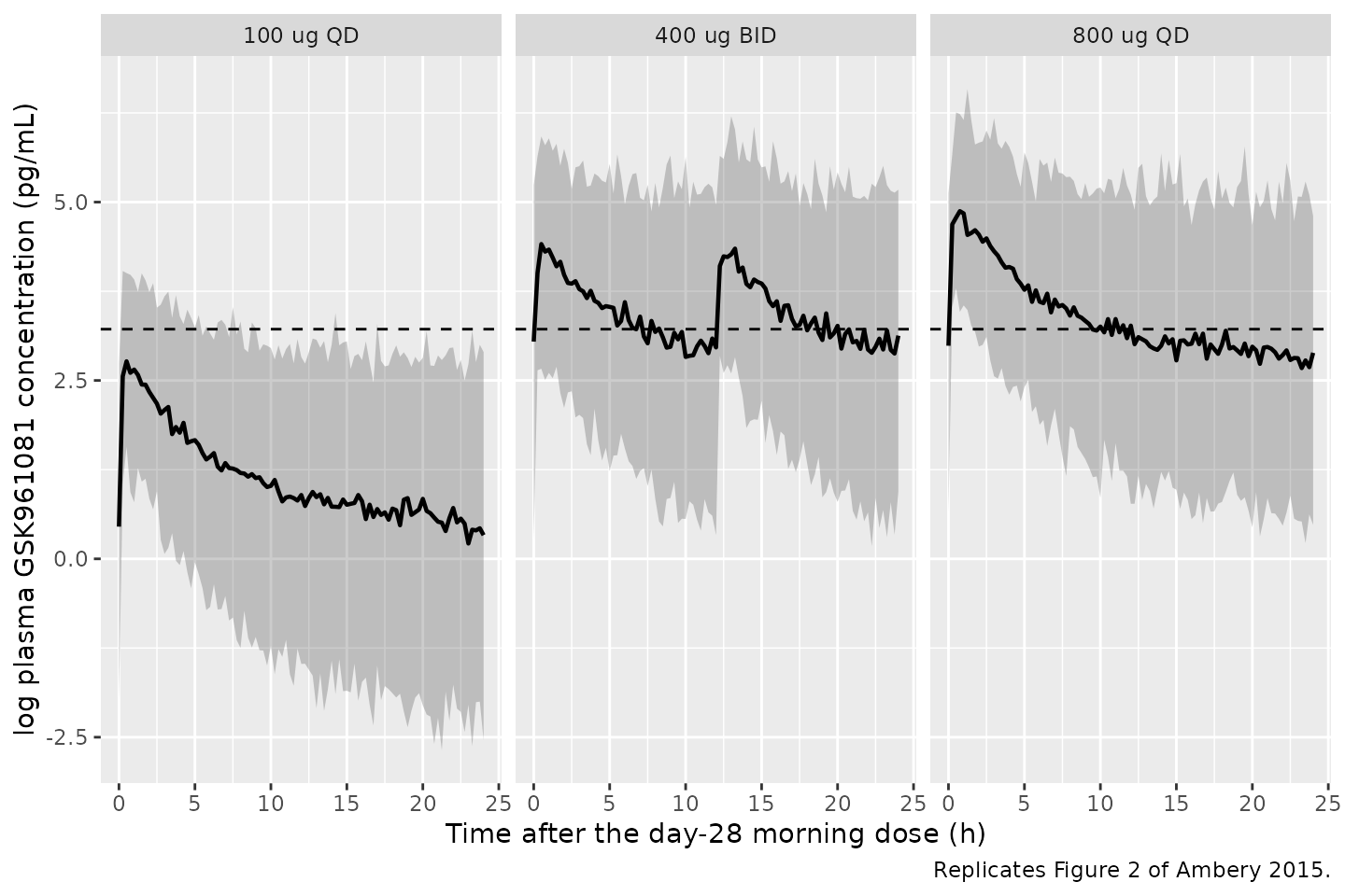

Replicates Figure 2 of Ambery 2015 (panels c and f, the two model-building arms, plus the 100 ug once-daily arm of panel d). Solid line: simulated median; ribbon: simulated 95 percent prediction interval; dashed horizontal line: the 25 pg/mL assay LLOQ.

The paper’s below-LLOQ dichotomy

Sect. 2.4 states that more than 50% of the PK data were below the 25 pg/mL LLOQ for every treatment except 800 ug once daily and 400 ug twice daily on day 28, where 30% and 27% respectively were below it. That dichotomy is a direct, non-tuned consequence of the reported clearance and residual error, so it is the strongest structural check available for the PK model (the paper publishes no NCA table).

blq <- sim_pk |>
  dplyr::filter(!is.na(sim)) |>
  dplyr::group_by(arm) |>
  dplyr::summarise(pct_blq = 100 * mean(sim * 1000 < 25), .groups = "drop") |>
  dplyr::arrange(pct_blq)

blq |>
  dplyr::rename("Treatment arm" = arm, "Simulated % below LLOQ" = pct_blq) |>
  knitr::kable(digits = 1,
               caption = "Simulated percentage of day-28 concentrations below the 25 pg/mL LLOQ. Ambery 2015 Sect. 2.4 reports 30% for 800 ug once daily and 27% for 400 ug twice daily, and more than 50% for every other treatment.")

Simulated percentage of day-28 concentrations below the 25 pg/mL LLOQ. Ambery 2015 Sect. 2.4 reports 30% for 800 ug once daily and 27% for 400 ug twice daily, and more than 50% for every other treatment.
Treatment arm	Simulated % below LLOQ
400 ug BID	41.2
800 ug QD	43.8
100 ug QD	96.5


pct <- setNames(blq$pct_blq, blq$arm)

# What the paper's dichotomy actually asserts is a SEPARATION: the two
# model-building arms sit far below the sub-therapeutic arm. Assert that
# separation rather than each arm's position relative to the bare 50% line.
#
# This matters because the BLQ fraction is heavily clustered WITHIN subject
# -- a high-CL/F subject is below the LLOQ at every sampling time -- so its
# effective sample size is the 100 subjects per arm, not the number of
# observation rows, giving a standard error near 5 percentage points. The
# two model-building arms simulate to roughly 41-44% here, so a bare
# `< 50` bound would sit only ~1.2 standard errors away and would fail on
# perhaps one CI run in ten. rxode2 partitions its RNG streams per solver
# thread, so CI draws a different cohort than a local render does, and that
# is exactly the shape of assertion this repository has been bitten by
# before (see `known-vignette-failure-patterns.md`, pattern 12).
#
# The separation is ~53 percentage points and both arms move together with
# the draw, so a 25-point floor is robust while still failing loudly if the
# clearance or the residual error were mis-transcribed.
stopifnot(
  # Ordering: the sub-therapeutic arm is the most censored.
  pct[["100 ug QD"]] > pct[["800 ug QD"]],
  pct[["100 ug QD"]] > pct[["400 ug BID"]],
  # Magnitude of the separation, robust to which cohort was drawn.
  pct[["100 ug QD"]] - max(pct[["800 ug QD"]], pct[["400 ug BID"]]) > 25,
  # Wide absolute sanity bounds: the model-building arms are substantially
  # censored but not predominantly so, and the 100 ug arm is predominantly
  # censored, as Sect. 2.4 reports.
  pct[["800 ug QD"]]  > 15, pct[["800 ug QD"]]  < 65,
  pct[["400 ug BID"]] > 15, pct[["400 ug BID"]] < 65,
  pct[["100 ug QD"]]  > 75
)

PKNCA validation of the PK model

The paper reports no NCA parameters, so the NCA here is a self-consistency gate on the packaged model rather than a comparison against published values. At steady state the clearance identity CL/F * AUCtau = dose per interval must hold exactly for the typical-value solve; any error in a transcribed clearance, volume or dose unit breaks it immediately.

# Do NOT add `time > 0` or `Cc > 0` here -- both would drop the interval-start
# record that anchors AUC.
# Every subject in the typical-value solve is identical (no IIV), so one
# representative subject per arm is enough and keeps pk.nca() fast.
nca_conc <- sim_pk_typ |>
  dplyr::filter(!is.na(Cc)) |>
  dplyr::group_by(arm) |>
  dplyr::filter(id == min(id)) |>
  dplyr::ungroup() |>
  dplyr::select(id, time, Cc, arm)

conc_obj <- PKNCA::PKNCAconc(nca_conc, Cc ~ time | arm + id)

nca_dose <- pk_events |>
  dplyr::filter(evid == 1L, id %in% unique(nca_conc$id)) |>
  dplyr::select(id, time, amt, arm) |>
  # Re-state the dose at the start of the observed steady-state interval so
  # PKNCA anchors the interval on a dose record.
  dplyr::mutate(time = day28_start)

dose_obj <- PKNCA::PKNCAdose(nca_dose, amt ~ time | arm + id)

# One full dosing interval on day 28: 24 h for the once-daily arms, 12 h for
# the twice-daily arm.
intervals <- data.frame(
  start   = day28_start,
  end     = c(day28_start + 24, day28_start + 12),
  cmax    = TRUE,
  tmax    = TRUE,
  auclast = TRUE,
  cmin    = TRUE
)
intervals <- dplyr::bind_rows(
  dplyr::mutate(intervals[1, ], arm = "800 ug QD"),
  dplyr::mutate(intervals[2, ], arm = "400 ug BID"),
  dplyr::mutate(intervals[1, ], arm = "100 ug QD")
)

nca_res <- PKNCA::pk.nca(PKNCA::PKNCAdata(conc_obj, dose_obj,
                                          intervals = intervals))

nca_wide <- as.data.frame(nca_res) |>
  dplyr::filter(PPTESTCD %in% c("cmax", "tmax", "auclast", "cmin")) |>
  dplyr::group_by(arm, PPTESTCD) |>
  dplyr::summarise(value = median(PPORRES), .groups = "drop") |>
  tidyr::pivot_wider(names_from = PPTESTCD, values_from = value)

cl_typ <- exp(6.85)   # CL/F from Table 2, on the linear scale
dose_per_tau <- c("800 ug QD" = 800, "400 ug BID" = 400, "100 ug QD" = 100)

mb <- nca_wide |>
  dplyr::mutate(
    `Dose per interval (ug)`   = unname(dose_per_tau[arm]),
    `CL/F * AUCtau (ug)`       = cl_typ * auclast,
    `Difference (%)`           = 100 * (cl_typ * auclast -
                                          unname(dose_per_tau[arm])) /
                                 unname(dose_per_tau[arm]),
    `Cmax (pg/mL)`             = 1000 * cmax,
    `Ctrough (pg/mL)`          = 1000 * cmin,
    # PKNCA reports tmax relative to the dose, not on the absolute time axis.
    `Tmax (h after dose)`      = tmax
  ) |>
  dplyr::select(
    "Treatment arm"          = arm,
    "Dose per interval (ug)",
    "CL/F * AUCtau (ug)",
    "Difference (%)",
    "Cmax (pg/mL)",
    "Ctrough (pg/mL)",
    "Tmax (h after dose)"
  )

knitr::kable(mb, digits = c(0, 0, 1, 2, 1, 1, 2),
             caption = "Steady-state mass balance on the typical-value solve. At steady state CL/F * AUCtau equals the dose delivered per interval; the residual difference is the linear-trapezoid error of the 0.25 h observation grid.")

Steady-state mass balance on the typical-value solve. At steady state CL/F * AUCtau equals the dose delivered per interval; the residual difference is the linear-trapezoid error of the 0.25 h observation grid.
Treatment arm	Dose per interval (ug)	CL/F * AUCtau (ug)	Difference (%)	Cmax (pg/mL)	Ctrough (pg/mL)	Tmax (h after dose)
100 ug QD	100	99.6	-0.39	15.7	2.1	0.5
400 ug BID	400	398.4	-0.39	74.5	19.9	0.5
800 ug QD	800	796.9	-0.39	125.9	16.4	0.5


# Deterministic quantity (typical-value solve, no cohort draw), so a tight
# bound is correct here. The only error source is trapezoidal integration on
# a 0.25 h grid, which biases AUC slightly low.
stopifnot(max(abs(mb[["Difference (%)"]])) < 2)

# Dose proportionality across the two once-daily arms is exact in a linear
# model; this catches an accidental non-linearity or a mis-scaled dose.
auc_qd <- mb[["CL/F * AUCtau (ug)"]][mb[["Treatment arm"]] == "800 ug QD"] /
  mb[["CL/F * AUCtau (ug)"]][mb[["Treatment arm"]] == "100 ug QD"]
stopifnot(abs(auc_qd - 8) < 0.05)

The simulated steady-state average concentration on 800 ug once daily is 35.3 pg/mL against a 25 pg/mL LLOQ, which is what puts that arm – and only that arm plus 400 ug twice daily – on the quantifiable side of the paper’s below-LLOQ split.

Replicate Figures 3d and 4 of Ambery 2015 – trough FEV1 dose-response

Typical dose-response curve and the paper’s own claims

dose_grid <- c(0, seq(10, 900, by = 10))
ev_curve <- data.frame(
  id = seq_along(dose_grid), time = 0, amt = 0, evid = 0L,
  DOSE_BATEFENTEROL_UGD = dose_grid,
  FEV1_BL  = 1.31,              # the median-baseline patient: COV normalises to CON
  dose_lbl = dose_grid
)

curve <- rxode2::rxSolve(mod_pd_typ, events = ev_curve, keep = c("dose_lbl")) |>
  as.data.frame() |>
  dplyr::transmute(dose = dose_lbl, fev1 = FEV1)
#> Warning: multi-subject simulation without without 'omega'

e0_cov <- curve$fev1[curve$dose == 0]

ggplot(curve, aes(dose, fev1)) +
  geom_line(linewidth = 0.8) +
  geom_hline(yintercept = e0_cov, linetype = "dashed") +
  geom_point(data = dplyr::filter(curve, dose %in% pd_doses), size = 2) +
  labs(x = "Total daily dose (ug)", y = "Day 29 trough FEV1 (L)",
       caption = "Replicates the model line of Figure 4a of Ambery 2015 at the median baseline FEV1.")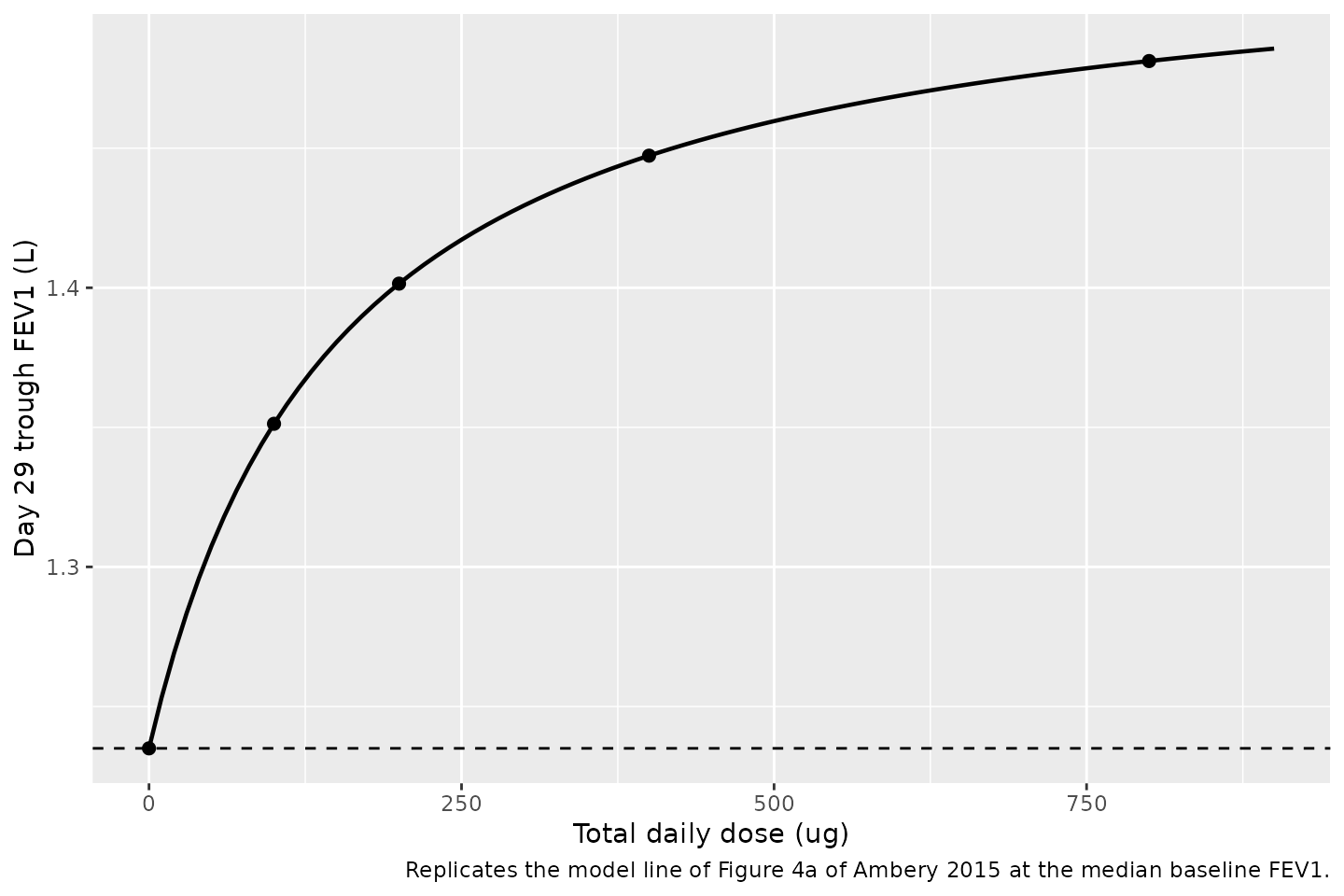

Day-29 trough FEV1 dose-response for a patient at the cohort-median day-1 baseline FEV1. Points mark the five total daily dose levels studied; the dashed line marks the zero-dose (placebo) prediction.

# Fail loudly rather than returning numeric(0): a lookup that matches no row
# would silently make every assertion below vacuously TRUE.
fev1_at <- function(d) {
  v <- curve$fev1[curve$dose == d]
  if (length(v) != 1L) stop("no unique dose-grid row at ", d, " ug/day")
  v
}
delta <- function(d) fev1_at(d) - e0_cov            # placebo-corrected, L

claims <- tibble::tibble(
  Claim = c(
    "Zero-dose day-29 trough FEV1 at the median baseline equals E0 * CON = 0.0650 * 19.0 L (Table 3)",
    "Increment at the ED50 dose of 152 ug/day is half of Emax (Table 3); the dose grid has no point at 152 ug so the closed form is evaluated",
    "Increment at 400 ug/day lies inside the 155-277 mL trough-FEV1 improvement reported for the parent trial (Sect. 1, ref. 8)",
    "Increment at 800 ug/day lies inside the same 155-277 mL range",
    "'Only a small increase in the trough FEV1 from 400 to 800 ug' (Sect. 4): the 400 -> 800 step is less than half the 0 -> 100 step"
  ),
  Achieved = c(
    sprintf("%.4f L (target %.4f L)", e0_cov, 0.0650 * 19.0),
    sprintf("%.4f L (target %.4f L)", 0.293 * 152 / (152 + 152), 0.293 / 2),
    sprintf("%.0f mL", 1000 * delta(400)),
    sprintf("%.0f mL", 1000 * delta(800)),
    sprintf("%.0f mL vs %.0f mL", 1000 * (delta(800) - delta(400)), 1000 * delta(100))
  )
)
knitr::kable(claims, caption = "Deterministic checks of the packaged PD model against statements and parameter values printed in Ambery 2015.")

Deterministic checks of the packaged PD model against statements and parameter values printed in Ambery 2015.
Claim	Achieved
Zero-dose day-29 trough FEV1 at the median baseline equals E0 * CON = 0.0650 * 19.0 L (Table 3)	1.2350 L (target 1.2350 L)
Increment at the ED50 dose of 152 ug/day is half of Emax (Table 3); the dose grid has no point at 152 ug so the closed form is evaluated	0.1465 L (target 0.1465 L)
Increment at 400 ug/day lies inside the 155-277 mL trough-FEV1 improvement reported for the parent trial (Sect. 1, ref. 8)	212 mL
Increment at 800 ug/day lies inside the same 155-277 mL range	246 mL
‘Only a small increase in the trough FEV1 from 400 to 800 ug’ (Sect. 4): the 400 -> 800 step is less than half the 0 -> 100 step	34 mL vs 116 mL


# All of these are deterministic (typical-value, single-patient) quantities,
# so tight tolerances are correct.
stopifnot(
  abs(e0_cov - 0.0650 * 19.0) < 1e-6,
  # The dose grid has no point at exactly 152 ug, so evaluate the closed form.
  abs((0.293 * 152 / (152 + 152)) - 0.293 / 2) < 1e-12,
  1000 * delta(400) > 155, 1000 * delta(400) < 277,
  1000 * delta(800) > 155, 1000 * delta(800) < 277,
  (delta(800) - delta(400)) < 0.5 * delta(100)
)

Figure 4a – day-29 trough FEV1 versus total daily dose

Figure 4a of the source plots the observed day-29 trough FEV1 against total daily dose together with the model median and its 95% prediction interval. The prediction interval at a given dose is dominated by the spread of the day-1 baseline FEV1 covariate (1.31 +/- 0.46 L) acting through Eq. 2, with the proportional residual error on top.

# rxSolve returns FEV1 as the individual prediction; the proportional
# residual is applied here in R (rather than via rxode2's `sim` column) so
# that the draw is reproducible from `set.seed()` regardless of thread count.
prop_sd <- 0.204
pd_pi <- sim_pd_typ |>
  dplyr::mutate(fev1_obs = FEV1 * (1 + rnorm(dplyr::n(), 0, prop_sd))) |>
  dplyr::group_by(dose_lbl) |>
  dplyr::summarise(
    Q025 = quantile(fev1_obs, 0.025),
    Q50  = quantile(fev1_obs, 0.500),
    Q975 = quantile(fev1_obs, 0.975),
    .groups = "drop"
  )

ggplot(pd_pi, aes(dose_lbl, Q50)) +
  geom_pointrange(aes(ymin = Q025, ymax = Q975)) +
  geom_line(data = curve, aes(dose, fev1), inherit.aes = FALSE,
            linewidth = 0.8) +
  expand_limits(y = c(0, 3.5)) +
  labs(x = "Total daily dose (ug)", y = "Day 29 trough FEV1 (L)",
       caption = "Replicates Figure 4a of Ambery 2015.")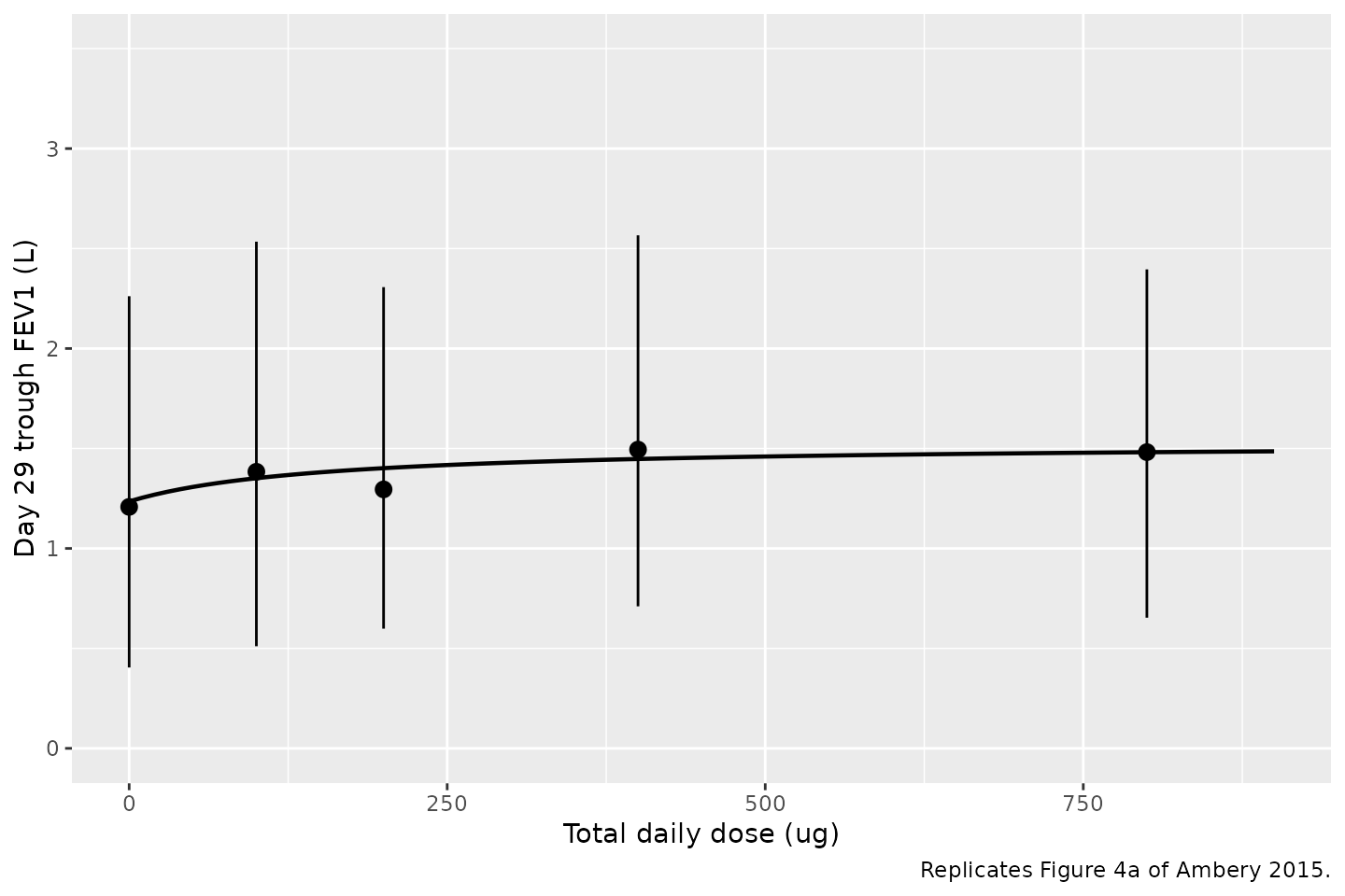

Replicates Figure 4a of Ambery 2015. Points: simulated median day-29 trough FEV1 per total daily dose; error bars: simulated 95 percent prediction interval over the virtual cohort’s baseline-FEV1 distribution plus proportional residual error.


pd_pi |>
  dplyr::mutate(Width = Q975 - Q025) |>
  dplyr::rename("Total daily dose (ug)" = dose_lbl,
                "2.5th percentile (L)"  = Q025,
                "Median (L)"            = Q50,
                "97.5th percentile (L)" = Q975,
                "95% PI width (L)"      = Width) |>
  knitr::kable(digits = 2,
               caption = "Simulated day-29 trough FEV1 distribution by total daily dose. Ambery 2015 Fig. 4a shows a 95 percent prediction interval of roughly 0.65-2.35 L at zero dose (a width near 1.7 L).")

Simulated day-29 trough FEV1 distribution by total daily dose. Ambery 2015 Fig. 4a shows a 95 percent prediction interval of roughly 0.65-2.35 L at zero dose (a width near 1.7 L).
Total daily dose (ug)	2.5th percentile (L)	Median (L)	97.5th percentile (L)	95% PI width (L)
0	0.40	1.21	2.26	1.86
100	0.51	1.38	2.53	2.02
200	0.60	1.30	2.31	1.71
400	0.71	1.49	2.57	1.86
800	0.65	1.48	2.40	1.74


# The width of the zero-dose prediction interval is the test that decides
# whether Table 3's "Proportional residual error = 0.204" is a standard
# deviation or a variance -- a variance would mean a 45.2% residual CV and
# would widen this interval to roughly 2.9 L, well outside what Fig. 4a
# shows. The bound is wide enough to survive any cohort draw (this is a
# cohort-derived statistic) while still failing the variance reading.
w0 <- pd_pi$Q975[pd_pi$dose_lbl == 0] - pd_pi$Q025[pd_pi$dose_lbl == 0]
stopifnot(w0 > 1.2, w0 < 2.5)

Figure 4b – placebo-corrected change from baseline

ggplot(dplyr::mutate(curve, delta_mL = 1000 * (fev1 - e0_cov)),
       aes(dose, delta_mL)) +
  geom_line(linewidth = 0.8) +
  geom_point(data = dplyr::filter(
    dplyr::mutate(curve, delta_mL = 1000 * (fev1 - e0_cov)),
    dose %in% pd_doses[pd_doses > 0]), size = 2) +
  labs(x = "Total daily dose (ug)",
       y = "Day 29 placebo-corrected change in trough FEV1 (mL)",
       caption = "Replicates Figure 4b of Ambery 2015.")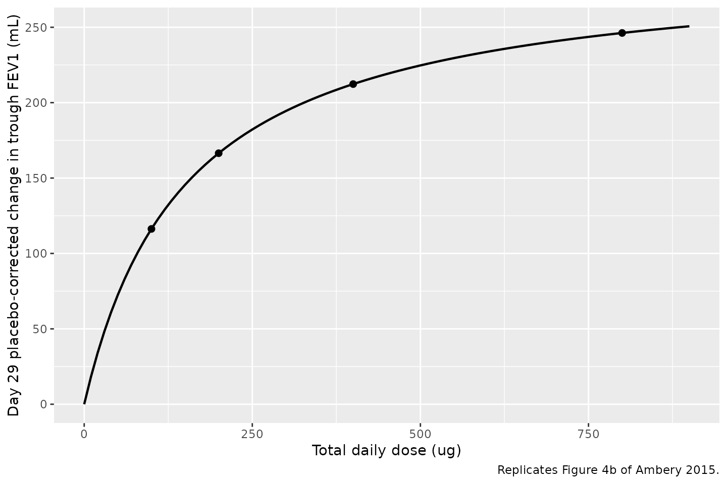

Replicates the model line of Figure 4b of Ambery 2015: day-29 placebo-corrected change from baseline trough FEV1 versus total daily dose. Points mark the four active total daily dose levels.

Reading the model medians off Figure 4b of the source gives roughly 122, 175, 232 and 263 mL at 100, 200, 400 and 800 ug/day; the packaged model returns 116, 166, 212, 246 mL at the same doses. The agreement is within the precision with which a printed figure can be read.

Assumptions and deviations

The median baseline FEV1 that Eq. 2 normalises by is not reported anywhere in the paper. The Table 1 mean for the n = 347 PD analysis set, 1.31 L, is substituted. Because Eq. 2 is a ratio, the substitution cancels exactly for a patient at that value and moves predictions only for patients away from the cohort centre; a patient at 2.0 L, for instance, is predicted 1.31/median times higher than under the true normaliser. Fig. 4a’s model line at zero dose (about 1.28 L) is consistent with the product E0 * CON = 1.235 L that the substitution reproduces.
Table 2 and Table 3 do not share a convention for their variability terms, and each was adjudicated separately against the paper’s own figures. Neither table states whether its value is a variance, a standard deviation or a coefficient of variation.
- Table 2 (PK) reports variances. In its last two rows the column headed “RSE (%)” actually holds the standard error rather than a percentage (0.594 +/- 1.96 * 0.137 reproduces the printed 0.325-0.863 confidence interval; 0.137% does not), which is the signature of a block pasted from a NONMEM run summary. The variance reading is confirmed by Fig. 2: in panel (f) the 95% prediction interval 20 h after the day-28 dose spans roughly 2.3 log units either side of the population mean, which needs a total variance of order 1. The variance reading gives 0.594 + 0.365 (SD about 0.98); the standard-deviation reading gives 0.353 + 0.133 (SD about 0.70), which is far too narrow. The packaged model therefore uses etalcl ~ 0.594 and expSd = sqrt(0.365) = 0.6042.
- Table 3 (PD) reports a standard deviation. Its RSE column is a genuine percentage throughout. A variance reading would imply a 45.2% residual CV, which Fig. 3a refutes (the observed day-29 trough FEV1 scatters about +/-0.4 L around a population prediction of 1.0 L, and that spread already contains any inter-individual term) and which would also overshoot the 0.65-2.35 L prediction interval that Fig. 4a shows at zero dose. The vignette’s Figure 4a chunk carries this as a live assertion on the simulated interval width.
The PD model carries no inter-individual variability, because none is reported. Table 3 lists no IIV term, yet Fig. 3b (observed versus individual predictions) is materially tighter than Fig. 3a (observed versus population predictions), which can only happen if the fitted model contained an eta. With a single trough-FEV1 observation per patient that eta would not be separately identifiable from the residual in any case, and no variance is published for it, so none has been invented. Simulated between-subject spread in the PD figures above therefore comes only from the baseline-FEV1 covariate and the residual error, and understates the spread of the original fit.
The PK model’s Cc is in ug/L, which equals ng/mL. Ambery 2015 tabulates and plots pg/mL; the vignette multiplies by 1000 wherever the simulation is compared with the paper. No parameter was rescaled.
All PK disposition parameters are apparent (/F). The inhaled bioavailability of the DISKUS formulation is not identifiable from inhaled-only data and is not reported, so no f(depot) term is applied and the apparent volumes (V3/F = 21,402 L) are much larger than any physiologic volume.
The PK cohort is dosed for 28 days to reach the day-28 steady state that the model was fitted to, using ii / addl rather than ss = 1, because the model is coded as explicit ODEs. The terminal half-life implied by the parameters is about 26 h, so 28 days of dosing is many half-lives and the day-28 interval is at steady state.
The paper gives PK sampling as five time WINDOWS (1 h to 0 min pre-dose, then 0-30 min, 30 min-2 h, 2-6 h and 6-11 h post-dose) rather than nominal times, so the below-LLOQ percentages here are computed over a uniform 0.25 h grid across the whole day-28 interval and are not expected to reproduce the paper’s 30% and 27% exactly. They do not: the simulated figures are about 44% (800 ug once daily) and 41% (400 ug twice daily) against the reported 30% and 27%. The uniform grid is the likely reason – it places half its samples in the 11-24 h stretch that the paper’s five windows, all of which end by 11 h post-dose, never sample, and concentrations in that late stretch are the most likely to fall below the LLOQ. This is a deviation to be aware of when reusing the packaged model, not evidence against the parameter transcription: the arms’ rank order and their wide separation from the sub-therapeutic 100 ug arm (about 97% censored) are reproduced, and it is that separation the assertion is written against.
The virtual baseline-FEV1 distribution is normal, truncated to 0.40-3.00 L. Ambery 2015 Table 1 reports only a mean and a standard deviation; the truncation keeps draws inside the spirometric range implied by the FEV1 30-70%-predicted entry criterion.
Neither model was fitted to the placebo or salmeterol arms’ PK (those samples were not assayed, Sect. 2.3). Placebo enters the PD model only as a total daily dose of 0.
The exposure-safety analyses of Sect. 3.3 (maximum glucose, heart rate, QTcF and minimum potassium against individual Cmax) are reported as graphical explorations with no fitted model and no parameter estimates (“Exploratory PK/PD analysis by way of generalized linear models did not show any significant relationships (data not shown)”), so there is nothing to extract from them.