Camostat / FOY-251 TMPRSS2 PK/PD against SARS-CoV-2 (Kosinsky 2022)
Source:vignettes/articles/Kosinsky_2022_camostat.Rmd
Kosinsky_2022_camostat.RmdModel and source
Kosinsky et al. (2022) built a semi-mechanistic PK/PD model for the oral serine protease inhibitor camostat mesylate and its active metabolite FOY-251, to predict inhibition of host TMPRSS2 and, through it, of SARS-CoV-2 cell entry. The paper contributes two packaged models:
-
Kosinsky_2022_camostat_invitro– the in-vitro PD model fit to cell-free recombinant TMPRSS2 activity and SARS-2-S pseudovirus entry (Hoffmann et al. 2020 data). It estimates the inhibition constantki, the half-maximal activityki50, and the Hill coefficient. -
Kosinsky_2022_camostat_pkpd– the in-vivo semi-mechanistic PK/PD model: one-compartment FOY-251 PK driving a TMPRSS2 covalent-inhibition turnover model, with the PD parameters carried from the in-vitro fit. It is used for the dose-regimen simulations.
inv <- readModelDb("Kosinsky_2022_camostat_invitro")
pkpd <- readModelDb("Kosinsky_2022_camostat_pkpd")- Citation: Kosinsky Y, Peskov K, Stanski DR, Wetmore D, Vinetz J. Semi-Mechanistic Pharmacokinetic-Pharmacodynamic Model of Camostat Mesylate-Predicted Efficacy against SARS-CoV-2 in COVID-19. Microbiol Spectr. 2022;10(2):e02167-21. doi:10.1128/spectrum.02167-21. PK parameters in Table 1; PD parameters in Table 2; the in-vivo PK/PD ODEs are Equations 1 and 5 of Materials and Methods.
- Article: https://doi.org/10.1128/spectrum.02167-21 (open access, CC BY 4.0)
- Supplement: publisher supplementary PDF (ELF-compartment extension, Figures S1-S4).
Population
The PK model was fit to digitised human FOY-251 plasma profiles: a 12-h intravenous infusion of camostat (Midgley et al. 1994, Xenobiotica 24:79-92) and a single oral dose from the FOIPAN package insert (Kosinsky 2022 Results, Figure S1). Because camostat is hydrolysed by plasma esterases too rapidly to quantify, FOY-251 is the only measured analyte. The FOY-251 volume of distribution (22.4 L) approximates the extracellular water space and the terminal half-life is about 0.6 h.
The PD parameters come from in-vitro experiments of Hoffmann et al. (2020): recombinant TMPRSS2 enzymatic activity after 1 h incubation with FOY-251, and SARS-2-S-driven pseudovirus entry after 2 h incubation. No subject-level cohort or between-subject variability was reported; the model is deterministic and used for dose-regimen simulations.
Both models expose this provenance through their
population metadata, e.g.
readModelDb("Kosinsky_2022_camostat_pkpd")()$population.
Source trace
In-vivo PK/PD model (Kosinsky_2022_camostat_pkpd):
| Equation / parameter | Value | Source location |
|---|---|---|
lka (ka) |
0.67 1/h | Table 1 (RSE 5.78%) |
lfdepot (F) |
0.051 | Table 1 (RSE 4.66%) |
lvc (Vd) |
22.36 L | Table 1 (RSE 7.07%) |
lkel (kel) |
1.22 1/h | Table 1 (RSE 4.70%) |
propSd |
0.14 | Table 1 (RSE 17.3%) |
lki (ki) |
45638.51 nM | Table 2 (RSE 7.46%) |
kcat (fixed) |
400 1/h | Table 2 (fixed) |
kdis (fixed) |
0.049 1/h | Table 2 (fixed; 14 h complex half-life) |
kdeg (fixed) |
0.0575 1/h | Methods = log(2)/12 h (assumed enzyme half-life) |
lki50 (Ksp) |
0.047 | Table 2 (RSE 42.4%) |
hill (h) |
0.59 | Table 2 (RSE 16.6%) |
d/dt(depot), d/dt(central)
|
n/a | Equation 1 |
d/dt(target), d/dt(complex)
|
n/a | Equation 5 |
viralentry (Hill) |
n/a | Equation 4 |
In-vitro model (Kosinsky_2022_camostat_invitro): the
same ki (estimated), kcat/kdis
(fixed), ki50, and hill, with additive
residual error addSd_tmprss2 = 0.0346 (Table 2 a1 = 3.46%)
and addSd_viralentry = 0.0758 (Table 2 a2 = 7.58%);
in-vitro ODEs are Equation 3 and the viral-entry link is Equation 4.
In-vitro model: TMPRSS2 inhibition and viral entry
The in-vitro model integrates the covalent-inhibition ODEs at a fixed
applied FOY-251 concentration (CONC_FOY251_NM), reading
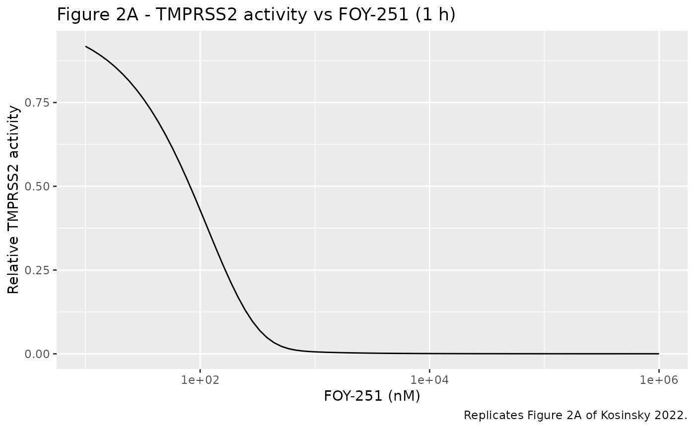
TMPRSS2 activity at 1 h and viral entry at 2 h. We sweep the applied
concentration to reproduce the dose-response relationships of Figure
2.
conc_grid <- 10^seq(1, 6, length.out = 80) # nM
obs_times <- c(0, 0.5, 1, 1.5, 2)
# This model has two `~` residual endpoints (TMPRSS2 activity and viral entry),
# so observation rows carry `cmt = "target"` (a real ODE state) with an explicit
# `dvid`, and `useLinCmt = FALSE` keeps the dvid mapping intact. rxSolve returns
# both `tmprss2` and `viralentry` as columns regardless. No dose is needed --
# the model sets target(0) = 1 internally.
ev_inv <- lapply(seq_along(conc_grid), function(i) {
  data.frame(
    id = i, time = obs_times, amt = NA_real_, cmt = "target",
    evid = 0L, dvid = 1L, CONC_FOY251_NM = conc_grid[i]
  )
}) |>
  dplyr::bind_rows()

sim_inv <- rxode2::rxSolve(inv, ev_inv, keep = "CONC_FOY251_NM", useLinCmt = FALSE) |>
  as.data.frame()
#> Warning: multi-subject simulation without without 'omega'

act_1h <- sim_inv |>
  dplyr::filter(abs(time - 1) < 1e-6) |>
  dplyr::transmute(conc = CONC_FOY251_NM, tmprss2_activity = tmprss2)
ve_2h <- sim_inv |>
  dplyr::filter(abs(time - 2) < 1e-6) |>
  dplyr::transmute(conc = CONC_FOY251_NM, viral_entry = viralentry)
# Replicates Figure 2A of Kosinsky 2022: recombinant TMPRSS2 activity (relative
# to control) versus FOY-251 concentration after 1 h incubation.
ggplot(act_1h, aes(conc, tmprss2_activity)) +
  geom_line() +
  scale_x_log10() +
  labs(
    x = "FOY-251 (nM)", y = "Relative TMPRSS2 activity",
    title = "Figure 2A - TMPRSS2 activity vs FOY-251 (1 h)",
    caption = "Replicates Figure 2A of Kosinsky 2022."
  )
# Replicates Figure 2C of Kosinsky 2022: viral entry rate as a function of the
# model-predicted remaining TMPRSS2 activity (Hill-Langmuir link, Equation 4).
act_grid <- tibble::tibble(sp = 10^seq(-3, 0, length.out = 200))
ksp <- 0.047
h <- 0.59
act_grid$viral_entry <- act_grid$sp^h / (act_grid$sp^h + ksp^h)
ggplot(act_grid, aes(sp, viral_entry)) +
  geom_line() +
  geom_vline(xintercept = ksp, linetype = "dashed") +
  scale_x_log10() +
  labs(
    x = "Relative TMPRSS2 activity", y = "Relative viral entry rate",
    title = "Figure 2C - viral entry vs TMPRSS2 activity",
    caption = "Dashed line: activity = ki50 = 0.047 (50% viral entry)."
  )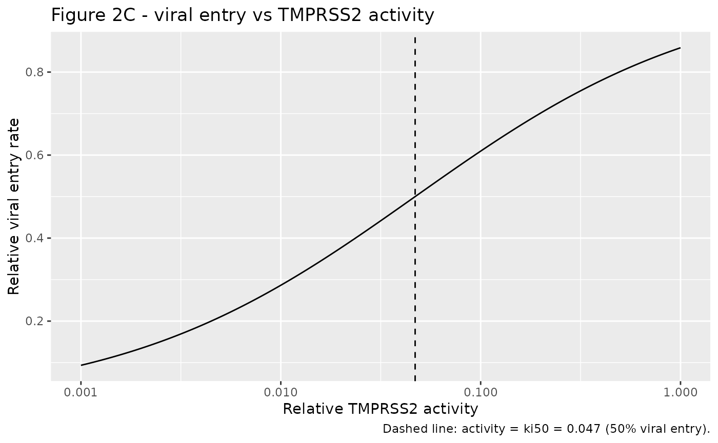
The key published claim is that about 95% inhibition of
TMPRSS2 is required for 50% inhibition of the viral entry rate.
By construction of the Hill-Langmuir half-maximum, viral entry equals
50% exactly when remaining TMPRSS2 activity equals ki50 =
0.047 (i.e. 95.3% TMPRSS2 inhibition).
ve_at_ki50 <- ksp^h / (ksp^h + ksp^h)
tmprss2_inhibition_at_half_entry <- 1 - ksp
stopifnot(
  # Half-maximal viral entry is at activity = ki50 (structural identity).
  abs(ve_at_ki50 - 0.5) < 1e-8,
  # which corresponds to ~95% TMPRSS2 inhibition.
  abs(tmprss2_inhibition_at_half_entry - 0.953) < 1e-3
)
ve_at_ki50
#> [1] 0.5
tmprss2_inhibition_at_half_entry
#> [1] 0.953
In-vivo PK/PD: dose-regimen simulations
The in-vivo model is simulated to steady state for each camostat dosing regimen. Camostat mesylate doses in mg are converted to FOY-251-equimolar nmol using the camostat mesylate molecular weight (494.52 g/mol; see Assumptions).
mw_camostat_mesylate <- 494.52 # g/mol (camostat mesylate salt, PubChem CID 5284360)
to_nmol <- function(mg) mg / mw_camostat_mesylate * 1e6

regimens <- tibble::tribble(
  ~regimen,    ~mg,  ~tau,
  "200 q8h",   200,  8,
  "200 q6h",   200,  6,
  "400 q6h",   400,  6,
  "600 q6h",   600,  6
)

sim_one <- function(mg, tau) {
  horizon <- 24 * 10
  t0 <- horizon - tau
  ev <- rxode2::et() |>
    rxode2::et(amt = to_nmol(mg), ii = tau, until = horizon, cmt = "depot") |>
    rxode2::et(seq(t0, horizon, length.out = 400))
  s <- rxode2::rxSolve(pkpd, ev, atol = 1e-10, rtol = 1e-8, maxsteps = 1e6)
  s[s$time >= t0, ]
}

time_avg <- function(x, t) {
  sum(diff(t) * (head(x, -1) + tail(x, -1)) / 2) / (max(t) - min(t))
}

ss_tab <- regimens |>
  rowwise() |>
  mutate(
    .sim = list(sim_one(mg, tau)),
    Cc_avg = time_avg(.sim$Cc, .sim$time),
    TMPRSS2_pct = time_avg(.sim$tmprss2, .sim$time),
    ViralEntry_pct = time_avg(.sim$viralentry, .sim$time)
  ) |>
  ungroup() |>
  select(regimen, Cc_avg, TMPRSS2_pct, ViralEntry_pct)
# Table 3 of Kosinsky 2022 (time-averaged model outcomes at steady state).
published3 <- tibble::tribble(
  ~regimen,  ~Cc_avg_pub, ~TMPRSS2_pub, ~ViralEntry_pub,
  "200 q8h",  96.6,        14.9,         64.2,
  "200 q6h",  129,         10.3,         59.9,
  "400 q6h",  258,         6.06,         51.5,
  "600 q6h",  386,         4.38,         46.4
)

cmp3 <- ss_tab |>
  left_join(published3, by = "regimen") |>
  mutate(
    Cc_pct_diff = 100 * (Cc_avg - Cc_avg_pub) / Cc_avg_pub,
    TMPRSS2_abs_diff = TMPRSS2_pct - TMPRSS2_pub,
    VE_abs_diff = ViralEntry_pct - ViralEntry_pub
  )

cmp3 |>
  transmute(
    Regimen = regimen,
    `Cc_avg sim (nM)` = round(Cc_avg, 1),
    `Cc_avg pub (nM)` = Cc_avg_pub,
    `TMPRSS2% sim` = round(TMPRSS2_pct, 2),
    `TMPRSS2% pub` = TMPRSS2_pub,
    `ViralEntry% sim` = round(ViralEntry_pct, 1),
    `ViralEntry% pub` = ViralEntry_pub
  ) |>
knitr::kable(caption = "Table 3 reproduction: time-averaged steady-state outcomes.")| Regimen | Cc_avg sim (nM) | Cc_avg pub (nM) | TMPRSS2% sim | TMPRSS2% pub | ViralEntry% sim | ViralEntry% pub |
|---|---|---|---|---|---|---|
| 200 q8h | 94.5 | 96.6 | 15.17 | 14.90 | 64.4 | 64.2 |
| 200 q6h | 126.0 | 129.0 | 10.43 | 10.30 | 60.2 | 59.9 |
| 400 q6h | 252.0 | 258.0 | 6.18 | 6.06 | 51.8 | 51.5 |
| 600 q6h | 378.0 | 386.0 | 4.48 | 4.38 | 46.7 | 46.4 |
# Deterministic model (no IIV): TMPRSS2 activity and viral entry reproduce the
# published values to within a fraction of a percentage point; Cc_avg is within
# a few percent (the residual is absorption-phase averaging detail not in the
# closed form). These are numerical bounds on a deterministic solve, so they
# are tight on purpose.
stopifnot(
  max(abs(cmp3$TMPRSS2_abs_diff)) < 0.5,
  max(abs(cmp3$VE_abs_diff)) < 0.5,
  max(abs(cmp3$Cc_pct_diff)) < 5
)
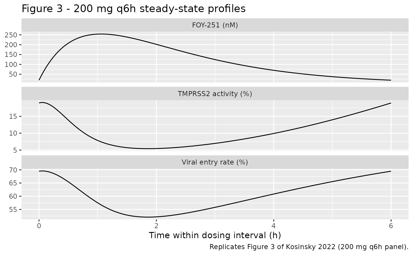
# Replicates Figure 3 of Kosinsky 2022: FOY-251 concentration, TMPRSS2 activity
# and viral entry rate over one steady-state dosing interval for 200 mg q6h.
prof <- sim_one(200, 6)
prof$t_rel <- prof$time - min(prof$time)
prof |>
  select(t_rel, Cc, tmprss2, viralentry) |>
  tidyr::pivot_longer(c(Cc, tmprss2, viralentry)) |>
  mutate(name = recode(name,
    Cc = "FOY-251 (nM)",
    tmprss2 = "TMPRSS2 activity (%)",
    viralentry = "Viral entry rate (%)"
  )) |>
  ggplot(aes(t_rel, value)) +
  geom_line() +
  facet_wrap(~name, scales = "free_y", ncol = 1) +
  labs(
    x = "Time within dosing interval (h)", y = NULL,
    title = "Figure 3 - 200 mg q6h steady-state profiles",
    caption = "Replicates Figure 3 of Kosinsky 2022 (200 mg q6h panel)."
  )
PKNCA validation (FOY-251 PK)
The published FOY-251 terminal elimination half-life
of about 0.6 h is the kel-governed disposition half-life
derived from the intravenous data. Because absorption is slower than
elimination (ka = 0.67 < kel = 1.22 1/h),
an oral profile shows flip-flop kinetics and its apparent terminal slope
reflects ka, not kel; so NCA is run here on an
intravenous bolus, which exposes the true elimination half-life.
ev_iv <- rxode2::et() |>
  rxode2::et(amt = to_nmol(200), cmt = "central") |>
  rxode2::et(seq(0, 8, length.out = 300))
sim_iv <- rxode2::rxSolve(pkpd, ev_iv)

sim_nca <- as.data.frame(sim_iv) |>
  dplyr::filter(!is.na(Cc)) |>
  dplyr::mutate(id = 1L, treatment = "200 mg IV bolus") |>
  dplyr::select(id, time, Cc, treatment)

conc_obj <- PKNCA::PKNCAconc(sim_nca, Cc ~ time | treatment + id)
dose_df <- data.frame(id = 1L, time = 0, amt = to_nmol(200), treatment = "200 mg IV bolus")
dose_obj <- PKNCA::PKNCAdose(dose_df, amt ~ time | treatment + id)
intervals <- data.frame(
  start = 0, end = Inf,
  cmax = TRUE, tmax = TRUE, aucinf.obs = TRUE, half.life = TRUE
)
nca_res <- PKNCA::pk.nca(PKNCA::PKNCAdata(conc_obj, dose_obj, intervals = intervals))
nca_wide <- tidyr::pivot_wider(
  as.data.frame(nca_res$result),
  id_cols = treatment, names_from = PPTESTCD, values_from = PPORRES
)
nca_wide |>
  dplyr::rename(
    "Treatment" = treatment,
    "Cmax (nM)" = cmax,
    "Tmax (h)" = tmax,
    "AUCinf (nM*h)" = aucinf.obs,
    "t1/2 (h)" = half.life
  ) |>
knitr::kable(caption = "PKNCA summary for a single 200 mg intravenous bolus.")| Treatment | Cmax (nM) | Tmax (h) | tlast | clast.obs | lambda.z | r.squared | adj.r.squared | lambda.z.time.first | lambda.z.time.last | lambda.z.n.points | clast.pred | t1/2 (h) | span.ratio | AUCinf (nM*h) |
|---|---|---|---|---|---|---|---|---|---|---|---|---|---|---|
| 200 mg IV bolus | 18087.32 | 0 | 8 | 1.043906 | 1.22 | 1 | 1 | 0.0267559 | 8 | 299 | 1.043906 | 0.5681535 | 14.03361 | 14825.69 |
Assumptions and deviations
- Camostat mesylate molecular weight (494.52 g/mol). The paper treats the camostat dose as equimolar to FOY-251 (Methods) but reports only the FOY-251 molecular weight (313 g/mol). To convert clinical mg doses of camostat mesylate to the model’s nmol dose, the maintainers used the camostat mesylate (salt) molecular weight of 494.52 g/mol (a standard chemical constant, PubChem CID 5284360). This value reproduces the published Table 3 Cc_avg to within a few percent across all simulated regimens, confirming the salt (rather than free-base) molecular weight is the correct one.
- In-vitro residual error scale. Table 2 reports the constant residual error parameters a1 (3.46%) and a2 (7.58%) as percentages. The maintainers encoded them as additive error on the fraction-of-baseline scale (0.0346 and 0.0758), matching the in-vitro readouts, which are relative activities.
-
TMPRSS2 enzyme half-life (12 h). The in-vivo
degradation rate
kdeg= 0.0575 1/h was computed by the authors from an assumed 12 h enzyme half-life (no literature estimate was available);ksynt=kdegfollows from the baseline activity being 1 (Equation 5). -
PD parameters shared across the two models.
ki,kcat,kdis,ki50, andhillwere estimated (or fixed) in the in-vitro model and reused as fixed inputs in the in-vivo PK/PD model, exactly as the authors did. - No between-subject variability. The model was fit to digitised literature profiles and used for deterministic simulations; no IIV or subject cohort was reported, so none was introduced.
-
ELF-compartment extension excluded. The supplement
adds an epithelial lining fluid compartment (parameters
ktr_elf,kel_elf) explored over four hypothetical scenarios (Figures S2-S4) rather than estimated from data. As a sensitivity exploration with no fitted parameters, it is not part of the packaged models. - No correction notice for this article was found as of 2026-10-01.