Paliperidone palmitate long-acting injectable (Yu 2025)
Source:vignettes/articles/Yu_2025_paliperidone.Rmd
Yu_2025_paliperidone.RmdModel and source
- Citation: Yu Y, et al. Prediction of drug concentrations in humans for long-acting injectable suspensions by a semi-mechanical muscle compartment model: a case study of paliperidone palmitate. Front Pharmacol. 2025;16:1507828. doi:10.3389/fphar.2025.1507828
- Description (dog): Preclinical (beagle dog). Semi-mechanistic intramuscular muscle-compartment model for paliperidone palmitate long-acting injectable nanocrystal suspensions (Yu 2025). The injected solid is split by mass into twelve particle-size bins; after a bin-specific lag time each bin dissolves into the injection-site fluid by the diffusion-layer model (particle number fixed, radius shrinking with the remaining mass, driving force = solubility minus the local dissolved concentration). Dissolved drug is carried to a one-compartment central disposition model by local blood flow. Covers the Invega Sustenna reference product and two Livzon test products (T1, T2) through formulation indicators that switch the bin particle sizes, bin lag times and bioavailability. Typical-value (deterministic) model.
- Description (human): Semi-mechanistic intramuscular muscle-compartment model for paliperidone palmitate long-acting injectable nanocrystal suspensions in humans, extrapolated from the beagle-dog model (Yu 2025). The injected solid is split by mass into twelve particle-size bins; after a bin-specific lag time each bin dissolves into the injection-site fluid by the diffusion-layer model (particle number fixed, radius shrinking with the remaining mass, driving force = solubility minus the local dissolved concentration). Dissolved drug is carried to a one-compartment central disposition model by local blood flow. Covers the Invega Sustenna reference product and two Livzon test products (T1, T2) through formulation indicators that switch the bin particle sizes, bin lag times and bioavailability. Bin lag times, particle sizes, bioavailability and physicochemistry are carried over from the dog model; the diffusion coefficient and the injection-site clearance are scaled by the human-to-dog muscle blood-flow ratio (73/350) and disposition is from Samtani 2009. Typical-value (deterministic) model.
- Article: https://doi.org/10.3389/fphar.2025.1507828
Yu 2025 built a semi-mechanistic “muscle compartment” model for intramuscular nanocrystal suspensions of paliperidone palmitate. The injected solid is split by mass into twelve particle-size bins (the 0-2, 2-5, 5-10, 10-20, …, 90-100 percent mass percentiles of the particle-size distribution). After a bin-specific lag time each bin dissolves into the injection-site fluid by the diffusion-layer model (Equation 1):
with the radius of a particle of bin , which shrinks as the bin dissolves while the particle count stays fixed. Dissolved drug is carried away by local blood flow (Equation 2) into a one-compartment central disposition model (Equation 3).
The model was first developed in beagle dogs for the Invega Sustenna reference suspension (R) and two Livzon test suspensions (T1, T2), with the bin lag times and bioavailability derived from the dog plasma profiles. It was then extrapolated to humans by replacing the disposition with Samtani 2009 values and scaling the diffusion coefficient and the injection-site clearance by the human-to-dog muscle blood-flow ratio (73/350). The package ships both:
-
Yu_2025_paliperidone_dog– the beagle-dog model; -
Yu_2025_paliperidone_human– the human extrapolation.
Both select the product with two indicators,
FORM_PALIPERIDONE_T1 and FORM_PALIPERIDONE_T2
(both 0 = reference R). One dose record into depot (mg) is
all that is needed; the model splits it across the bins.
Population
Dogs (Section 2.5.1): male beagle dogs, 7-9 months old, 9-11 kg, each given one intramuscular buttock injection of 50 mg paliperidone palmitate as R, T1 or T2, with plasma sampled to 36 days. The number of dogs per product is not reported.
Humans (Sections 2.6.2 and 3.3): no human data were fitted. The authors simulated 300 virtual individuals after a single 50 mg injection and compared product R against the mean profile reported by Samtani 2009.
The same information is available programmatically via
readModelDb("Yu_2025_paliperidone_dog")()$population and
readModelDb("Yu_2025_paliperidone_human")()$population.
Source trace
| Equation / parameter | Dog value | Human value | Source location |
|---|---|---|---|
Equation 1: d/dt(depot),
d/dt(diss_bin<n>)
|
n/a | n/a | Equation 1 |
Equation 2: d/dt(injsite)
|
n/a | n/a | Equation 2 |
Equation 3: d/dt(central)
|
n/a | n/a | Equation 3 |
lkel (1/h) |
log(ln 2 / 7.6) = log(0.0912) | log(0.0127) | Dog: Section 3.1.2 / Table 1 half-life 7.6 h; human: Table 4 |
lvc (L) |
log(8.5) | log(391) | Table 1 / Table 6; Table 4 |
lcltrans (mL/h) |
log(35) | log(7.3) | Table 1 CLdist; Table 4 CLtrans (see deviations: printed as L/h) |
lvregion (mL) |
log(0.5) | log(0.5) | Section 3.1.1 |
ldcoef (m^2/s) |
log(4.69e-12) | log(9.78e-13) | Section 3.3; Table 4 |
lhdl (um) |
log(3) | log(3) | Table 1 |
rho (g/cm^3) |
1.2 | 1.2 | Table 1 |
sol (mg/mL) |
0.00704 | 0.00704 | Table 1 |
lfdepot, lfdepot_t1,
lfdepot_t2
|
log(1), log(0.83), log(0.72) | same | Table 6 |
frac_bin1 … frac_bin12
|
0.02, 0.03, 0.05, 0.10 x 9 | same | Section 2.6.1 |
rad_bin<n>, rad_t1_bin<n>,
rad_t2_bin<n> (um) |
Table 7 rows R, T1, T2 | same | Table 7 |
tlag_bin<n>, tlag_t1_bin<n>,
tlag_t2_bin<n> (h) |
Table 2 rows R, T1, T2 | same | Table 2 |
Simulation
The model is deterministic (the paper reports no between-subject variability or residual error), so one subject per product reproduces the typical profiles.
mod_dog <- readModelDb("Yu_2025_paliperidone_dog")
mod_hum <- readModelDb("Yu_2025_paliperidone_human")

products <- tibble::tibble(
  id = 1:3,
  product = c("R", "T1", "T2"),
  FORM_PALIPERIDONE_T1 = c(0L, 1L, 0L),
  FORM_PALIPERIDONE_T2 = c(0L, 0L, 1L)
)

make_events <- function(obs_times) {
  dose <- products |>
    mutate(time = 0, amt = 50, evid = 1L, cmt = "depot")
  obs <- tidyr::crossing(products, time = obs_times) |>
    mutate(amt = 0, evid = 0L, cmt = "central")
  bind_rows(dose, obs) |>
    arrange(id, time, desc(evid)) |>
    as.data.frame()
}

# Dog: 36 days (last sampling day); human: 126 days (last Samtani 2009
# observation in Figure 5).
ev_dog <- make_events(seq(0, 36 * 24, by = 1))
ev_hum <- make_events(seq(0, 126 * 24, by = 2))

sim_dog <- rxode2::rxSolve(mod_dog, events = ev_dog, keep = "product") |>
  as.data.frame()
sim_hum <- rxode2::rxSolve(mod_hum, events = ev_hum, keep = "product") |>
  as.data.frame()
Replicate published figures
Dog model (Figures 4 and 6)
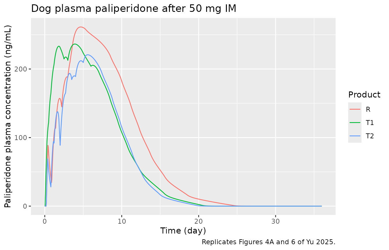
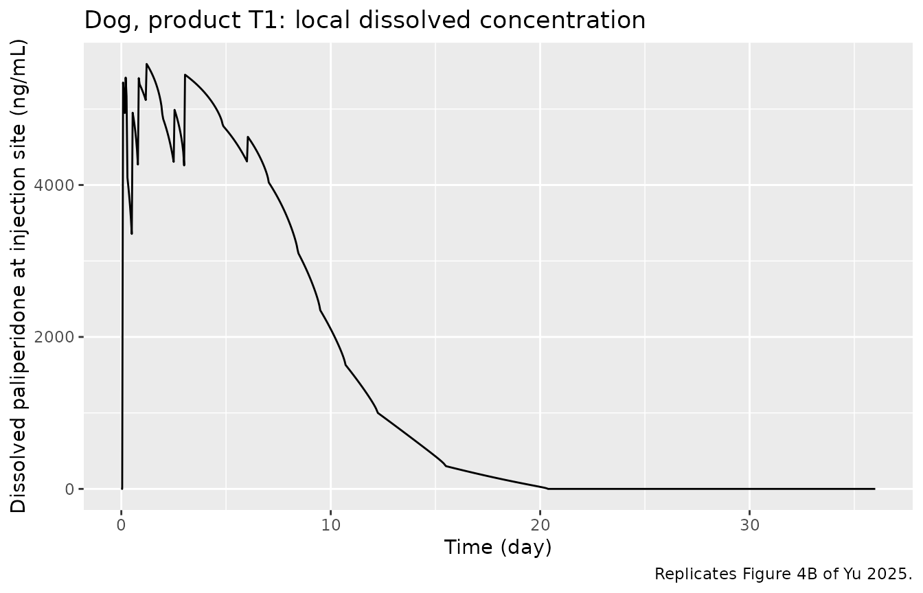
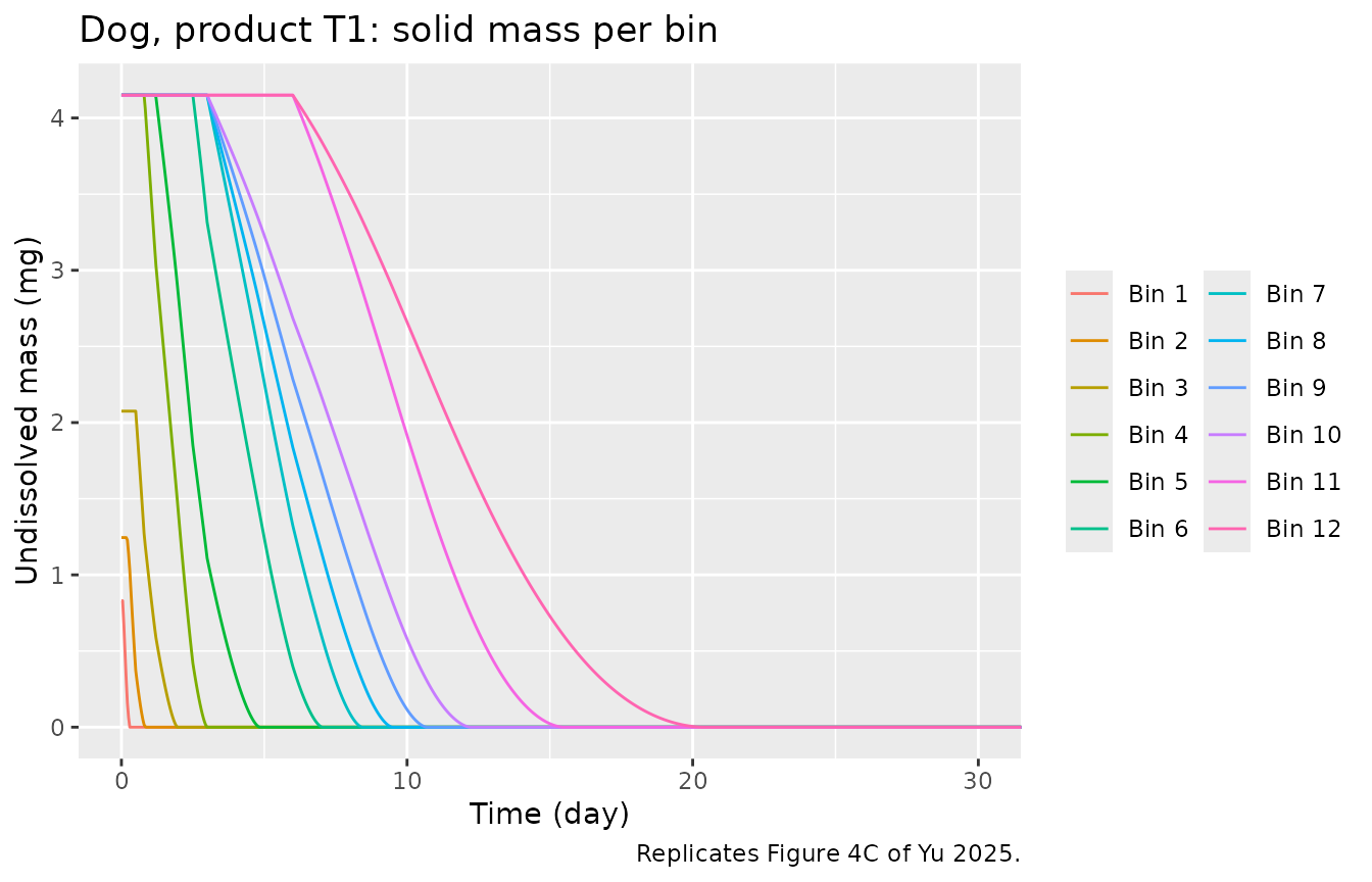
Figure 4 of the paper is labelled as the reference sample, but its plasma panel is identical to Figure 6A (T1), and its solid-mass panel starts each 10 percent bin at about 4.15 mg (= 0.83 x 50 mg x 0.10, the T1 bioavailability) with bins 11 and 12 starting to dissolve at day 6 (the T1 lag time of 144 h). It is therefore reproduced here with T1.
# Replicates Figure 4A / 6A (T1) and Figure 6B (T2) of Yu 2025, plus R.
ggplot(sim_dog, aes(time / 24, Cc, colour = product)) +
  geom_line() +
  labs(
    x = "Time (day)", y = "Paliperidone plasma concentration (ng/mL)",
    colour = "Product",
    title = "Dog plasma paliperidone after 50 mg IM",
    caption = "Replicates Figures 4A and 6 of Yu 2025."
  )
# Replicates Figure 4B of Yu 2025: dissolved paliperidone at the injection site.
sim_dog |>
  filter(product == "T1") |>
  ggplot(aes(time / 24, Cinj)) +
  geom_line() +
  labs(
    x = "Time (day)", y = "Dissolved paliperidone at injection site (ng/mL)",
    title = "Dog, product T1: local dissolved concentration",
    caption = "Replicates Figure 4B of Yu 2025."
  )
# Replicates Figure 4C of Yu 2025: undissolved solid mass in each bin. The
# solid left in bin n is its starting mass (frac_bin<n> x F x dose) minus
# what it has released.
frac <- c(0.02, 0.03, 0.05, rep(0.10, 9))
solid_t1 <- sim_dog |>
  filter(product == "T1") |>
  select(time, starts_with("diss_bin")) |>
  pivot_longer(-time, names_to = "bin", values_to = "dissolved") |>
  mutate(
    n = as.integer(sub("diss_bin", "", bin)),
    solid = frac[n] * 0.83 * 50 - dissolved,
    bin = factor(paste("Bin", n), levels = paste("Bin", 1:12))
  )
ggplot(solid_t1, aes(time / 24, solid, colour = bin)) +
  geom_line() +
  coord_cartesian(xlim = c(0, 30)) +
  guides(colour = guide_legend(ncol = 2)) +
  labs(
    x = "Time (day)", y = "Undissolved mass (mg)", colour = NULL,
    title = "Dog, product T1: solid mass per bin",
    caption = "Replicates Figure 4C of Yu 2025."
  )
Human model (Figures 5 and 7)
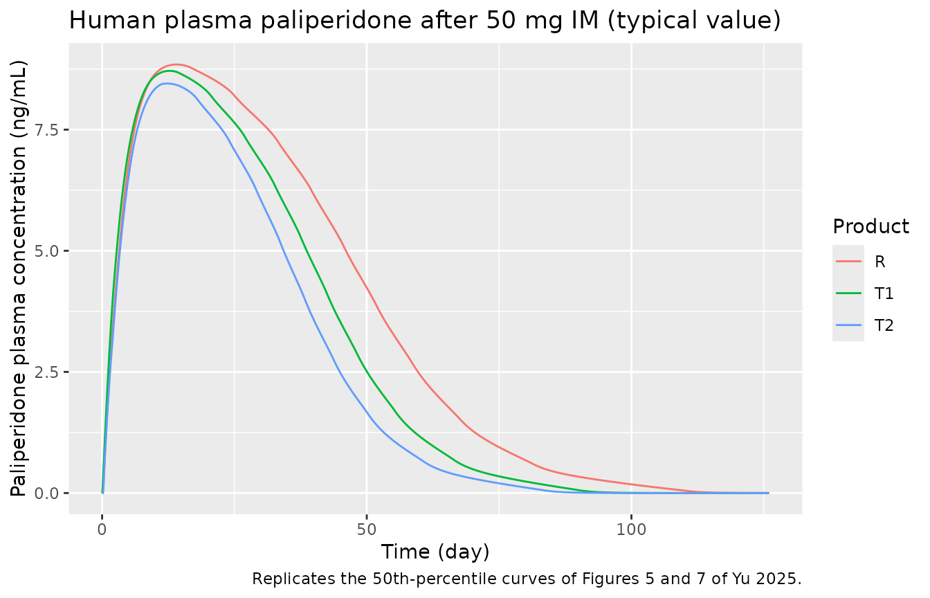
# Replicates the median curves of Figure 5 (R) and Figure 7 (T1, T2).
ggplot(sim_hum, aes(time / 24, Cc, colour = product)) +
  geom_line() +
  labs(
    x = "Time (day)", y = "Paliperidone plasma concentration (ng/mL)",
    colour = "Product",
    title = "Human plasma paliperidone after 50 mg IM (typical value)",
    caption = "Replicates the 50th-percentile curves of Figures 5 and 7 of Yu 2025."
  )
PKNCA validation
AUC0-t is computed over the paper’s windows: 0-36 days for the dogs (Table 3) and 0-126 days for humans (Table 5, the last Samtani 2009 observation).
run_nca <- function(sim, events, tend) {
  conc <- sim |>
    filter(!is.na(Cc)) |>
    select(id, time, Cc, product)
  conc <- bind_rows(
    conc,
    conc |> distinct(id, product) |> mutate(time = 0, Cc = 0)
  ) |>
    distinct(id, product, time, .keep_all = TRUE) |>
    arrange(id, product, time)
  dose <- events |>
    filter(evid == 1) |>
    select(id, time, amt, product)
  intervals <- data.frame(start = 0, end = tend, cmax = TRUE, tmax = TRUE, auclast = TRUE)
  PKNCA::pk.nca(PKNCA::PKNCAdata(
    PKNCA::PKNCAconc(conc, Cc ~ time | product + id),
    PKNCA::PKNCAdose(dose, amt ~ time | product + id),
    intervals = intervals
  ))
}
nca_dog <- run_nca(sim_dog, ev_dog, 36 * 24)
nca_hum <- run_nca(sim_hum, ev_hum, 126 * 24)
Comparison against published values
The reference values are the paper’s own simulated AUC0-t and Cmax (Tables 3 and 5), which is what a correct implementation should reproduce. The observed values are listed in the text below.
published_dog <- tibble::tribble(
  ~product, ~auclast, ~cmax,
  "R",      64962,    262.7,
  "T1",     53963,    225.8,
  "T2",     46808,    209.9
)
cmp_dog <- nlmixr2lib::ncaComparisonTable(
  simulated = nca_dog,
  reference = published_dog,
  by = "product",
  units = c(auclast = "ng*h/mL", cmax = "ng/mL"),
  tolerance_pct = 20
)
knitr::kable(cmp_dog, caption = "Dog: simulated vs. Yu 2025 Table 3 simulated values. * differs by >20%.")| NCA parameter | product | Reference | Simulated | % diff |
|---|---|---|---|---|
| Cmax (ng/mL) | R | 263 | 261 | -0.5% |
| Cmax (ng/mL) | T1 | 226 | 236 | +4.7% |
| Cmax (ng/mL) | T2 | 210 | 221 | +5.2% |
| AUClast (ng*h/mL) | R | 65000 | 64500 | -0.7% |
| AUClast (ng*h/mL) | T1 | 54000 | 53500 | -0.8% |
| AUClast (ng*h/mL) | T2 | 46800 | 46400 | -0.8% |
published_hum <- tibble::tribble(
  ~product, ~auclast, ~cmax,
  "R",      10009,    8.605,
  "T1",     8324,     8.234,
  "T2",     7220,     7.877
)
cmp_hum <- nlmixr2lib::ncaComparisonTable(
  simulated = nca_hum,
  reference = published_hum,
  by = "product",
  units = c(auclast = "ng*h/mL", cmax = "ng/mL"),
  tolerance_pct = 20
)
knitr::kable(cmp_hum, caption = "Human: simulated vs. Yu 2025 Table 5 simulated values. * differs by >20%.")| NCA parameter | product | Reference | Simulated | % diff |
|---|---|---|---|---|
| Cmax (ng/mL) | R | 8.6 | 8.84 | +2.8% |
| Cmax (ng/mL) | T1 | 8.23 | 8.71 | +5.8% |
| Cmax (ng/mL) | T2 | 7.88 | 8.45 | +7.3% |
| AUClast (ng*h/mL) | R | 10000 | 10100 | +0.6% |
| AUClast (ng*h/mL) | T1 | 8320 | 8360 | +0.4% |
| AUClast (ng*h/mL) | T2 | 7220 | 7250 | +0.4% |
Observed values for comparison: in dogs, AUC0-t 59,753 / 53,546 / 44,581 ngh/mL and Cmax 286.0 / 221.0 / 194.0 ng/mL for R / T1 / T2 (Table 3); in humans, Samtani 2009 reports AUC0-t 10,062 ngh/mL and Cmax 9.257 ng/mL for product R (Table 5).
nca_tab <- function(res) {
  as.data.frame(res) |>
    filter(PPTESTCD %in% c("auclast", "cmax")) |>
    select(product, PPTESTCD, PPORRES) |>
    pivot_wider(names_from = PPTESTCD, values_from = PPORRES)
}
chk_dog <- nca_tab(nca_dog) |> left_join(published_dog, by = "product", suffix = c("_sim", "_pub"))
chk_hum <- nca_tab(nca_hum) |> left_join(published_hum, by = "product", suffix = c("_sim", "_pub"))
chk <- bind_rows(chk_dog, chk_hum)
# Deterministic model, no random draws, so these hold on any machine.
# AUC0-t is fixed by F x dose / CL and lands within 1%; the per-bin
# dissolution shapes the peak, where the realised differences are
# 0.5-5% (dog) and 3-7% (human).
stopifnot(
  all(abs(chk$auclast_sim / chk$auclast_pub - 1) < 0.02),
  all(abs(chk$cmax_sim / chk$cmax_pub - 1) < 0.10)
)
Mass balance
Everything injected (F x dose) is eventually absorbed and eliminated, so the area under the curve to infinity equals F x dose / CL. The 126-day human window holds essentially all of it.
kel_h <- 0.0127
vc_h <- 391
auc_expected <- c(R = 1, T1 = 0.83, T2 = 0.72) * 50 / (kel_h * vc_h) * 1000
auc_sim <- nca_tab(nca_hum)
auc_sim$expected <- auc_expected[auc_sim$product]
knitr::kable(auc_sim |> select(product, auclast, expected),
  caption = "Human AUC0-126 day vs. F x dose / CL (ng*h/mL)", digits = 0
)| product | auclast | expected |
|---|---|---|
| R | 10069 | 10069 |
| T1 | 8357 | 8357 |
| T2 | 7250 | 7250 |
Assumptions and deviations
The paper’s printed values contain several inconsistencies. Each was resolved by the paper’s own simulated outputs (Tables 3 and 5, Figure 4), not by fitting:
-
Dog elimination rate constant. Table 1 prints
Ke,dog = 0.0693 /hbut states it was calculated from the 7.6 h half-life, which gives ln 2 / 7.6 = 0.0912 /h (0.0693 /h is ln 2 / 10 h). With F x dose / (ke x Vd) the half-life value reproduces the simulated AUC0-t of Table 3 for all three products to within 1%, while 0.0693 /h overpredicts it by about 30%. The model uses ln 2 / 7.6. - Dog diffusion coefficient. Table 1 and Section 3.1.1 give a fitted dog value of 1.17e-11 m^2/s, but the human derivation in Section 3.3 scales a dog value of 4.69e-12 m^2/s ((73/350) x 4.69e-12 = 9.78e-13, the Table 4 human value). The 4.69e-12 value reproduces the Table 3 Cmax values and Figure 4B/4C; 1.17e-11 overpredicts Cmax by 10-23%. The dog model uses 4.69e-12 m^2/s.
-
Injection-site clearance units. Table 1 gives
CLdist = 35 L/hand Table 4CLtrans = 7.3 L/h. With the 0.5 mL injection-site volume, a clearance of 35 L/h would keep the local dissolved concentration near 30 ng/mL and give a dog Cmax 1.8-3.5 times that of Table 3. Figure 4B shows local dissolved concentrations near 5000 ng/mL, which requires 35 mL/h. Both values are therefore used in mL/h. - Particle size as radius. Table 7 reports a “particle size” per bin. Used as the particle radius in Equation 1, the bin sizes reproduce Table 3 Cmax to within 5% and the bin dissolution times of Figure 4C (bins 11 and 12 of T1 start at day 6 and are gone by about day 15 and 20). Used as a diameter they make every bin dissolve about twice as fast and overpredict dog Cmax by 11-24%. The model uses them as radii.
-
Equation 1 particle count. As printed, the cube
root in Equation 1 is
(3 Solid_n / (4 pi rho))^(1/3), the radius of one sphere holding the whole bin mass; multiplied byN_nthis gives near-instantaneous dissolution. The model uses the standard diffusion-layer form, in which the radius is that of one particle,(3 Solid_n / (4 pi rho N_n))^(1/3), withN_nfixed by the starting bin mass and particle size. - Figure 4 product. Figure 4 is captioned with the reference sample, but its panels match product T1 (see above).
- Human parameters carried over from the dog. Diffusion-layer thickness, solid density, solubility, injection-site volume, the bin lag times and the bioavailabilities have no human values in the paper; the model carries the dog values over, as the paper describes. The human T1 and T2 AUC0-t of Table 5 are 0.83 and 0.72 times that of R, which confirms the carried-over bioavailabilities.
- Variability not reported. The paper simulated 300 virtual humans and shows 5th-95th percentile bands (Figures 5 and 7), but does not report which parameters varied or by how much. Both models are typical-value models with no random effects or residual error. The paper’s median curves have a slower terminal decline (for example 0.6 and 0.4 ng/mL at day 75 for T1 and T2, versus about 0.3 and 0.2 ng/mL here), as expected when variable absorption is summarised by a median; Table 5 Cmax is reproduced to within 3-7%.
- Dose. The 50 mg dose is treated as 50 mg of paliperidone, as in the paper: the human AUC of Table 5 equals 50 mg / CL with the Samtani 2009 clearance. Hydrolysis of the palmitate ester is not modelled.
-
Repeated injections. The model was published for a
single injection. A second dose into
depotis pooled with what remains of the first, and the bin lag times restart from the latest injection, so multiple-dose simulations are an extrapolation of the published model.