Model and source
- Citation: Yu B, Mei K, Zhan D, Tang Q, Cai H, Zhang R. Establishment of a Vancomycin Population Pharmacokinetic Model for Pediatric Patients Based on the Non-Linear Mixed-Effects Model. Drugs R D. 2025;25:309-320. doi:10.1007/s40268-025-00523-8
- Description: One-compartment IV population PK model for vancomycin in Chinese pediatric patients (birth to 15 years) receiving intermittent intravenous infusions and monitored by steady-state trough concentrations (Yu 2025). Clearance scales allometrically with body weight (fixed exponent 0.75, reference 70 kg) and as a power function of Schwartz-estimated GFR (estimated exponent 0.812, reference 173.42 mL/min/1.73 m^2); volume of distribution scales linearly with body weight (fixed exponent 1, reference 70 kg). Interindividual variability was estimable only on clearance; the proportional residual error was fixed at 30%.
- Article (open access): https://doi.org/10.1007/s40268-025-00523-8
- No supplementary material accompanies the article; the Code Availability statement offers the NONMEM code on request from the corresponding author.
Yu 2025 is a single-center retrospective therapeutic-drug-monitoring study of IV vancomycin in Chinese children. It has two quantitative products, and this vignette exercises both:
-
A one-compartment population PK model (Table 3,
with the parameter equations in Eqs. 12 and 13) - the model packaged
here as
Yu_2025_vancomycin. - A Monte Carlo simulation of steady-state trough concentrations across three renal-function strata and two guideline dosing regimens (Table 4, plotted in Fig. 3).
The first reproduces exactly. The second does not reproduce for the two renal-impairment strata, and the section “Table 4 does not follow from Eq. 12 for the impaired strata” below localizes why.
Population
The model was fit to 100 pediatric inpatients contributing 124 vancomycin concentrations at Anhui Provincial Children’s Hospital (Hefei, Anhui, China) between September 2021 and November 2023 (Yu 2025 Sect. 2.1, Table 1). Median age was 4 years (mean 5.17; range 0.0027-15), median actual body weight 24 kg (mean 21.49; range 1.25-74), and median height 106.5 cm (range 37-178); 41% were female. Median Schwartz eGFR was 173.42 mL/min/1.73 m^2 (mean 163.83; range 31.9-260.82), i.e. this cohort’s renal function skews supranormal, which matters below because the model’s eGFR reference is that same 173.42.
Patients on renal replacement therapy or ECMO, with undetectable vancomycin concentrations, or with incomplete clinical data were excluded. Dosing was empirical and clinician-chosen; vancomycin was given as a 60-minute IV intermittent infusion. Sampling was sparse and dominated by steady-state troughs drawn 30 minutes before the fourth dose, giving only 124 concentrations from 100 patients - barely more than one sample per subject. Plasma vancomycin was measured by enzyme amplification immunoassay (Siemens Viva-ProE) with a lower limit of quantification of 2 mg/L; measurable samples below the LLOQ were kept.
That sampling design drives three structural decisions in the paper that a user of this model needs to know about: a two-compartment model could not be supported, interindividual variability on volume was dropped as unestimable, and the residual error magnitude was fixed rather than estimated.
The same information is available programmatically via the model’s
population metadata
(readModelDb("Yu_2025_vancomycin")()$population).
Source trace
Per-parameter origin is recorded as an in-file comment next to each
ini() entry in
inst/modeldb/specificDrugs/Yu_2025_vancomycin.R. The table
below collects them in one place.
| Equation / parameter | Value | Source location |
|---|---|---|
lcl (CL at WT 70 kg, eGFR 173.42) |
8.22 L/h (RSE 9%) | Yu 2025 Table 3, theta_CL row |
lvc (V at WT 70 kg) |
113 L (RSE 18%) | Yu 2025 Table 3, theta_V row |
e_wt_cl |
0.75, fixed | Yu 2025 Eq. 8 CL_i = CL_pop * (WT/70)^0.75 and Eq. 12;
Sect. 2.4.1 “Clearance and V were scaled using fixed exponents of 0.75
and 1.0” |
e_wt_vc |
1, fixed | Yu 2025 Eq. 9 V_i = V_pop * (WT/70) and Eq. 13; same
Sect. 2.4.1 sentence |
e_crcl_cl |
0.812 (RSE 15%) | Yu 2025 Table 3, theta_GFR row; applied as
(GFR/173.42)^theta_GFR in Eq. 12 |
| Reference weight | 70 kg | Yu 2025 Eqs. 8, 9, 12, 13; confirmed in Sect. 4, which divides 8.22 L/h by 70 kg to obtain 0.117 L/h/kg |
| Reference eGFR | 173.42 mL/min/1.73 m^2 | Yu 2025 Eq. 12; equals the Table 1 cohort median, per Sect. 2.4.2 (“standardized by the median”) |
| eGFR definition | k * height (cm) / Scr (mg/dL) |
Yu 2025 Eq. 2 (Schwartz), with k in {0.33, 0.45, 0.55,
0.7} by age and sex; Eq. 1 gives the creatinine conversion 1 mg/dL =
88.4 umol/L |
etalcl |
omega^2 = 0.319225 | Yu 2025 Table 3: omega_CL 56.5% (RSE 10%); Eq. 3 gives
the exponential model P_i = theta_P * exp(eta_i)
|
| IIV on V | absent | Yu 2025 Sect. 3.2.1: “Because the estimated value of the inter-individual variability in V was too small, it was omitted in subsequent calculations” |
propSd |
0.3, fixed | Yu 2025 Table 3: residual unexplained variability 30% (fixed); Sect. 3.2.1 selected the proportional model (Eq. 5); Sect. 4 describes the 0.2/0.3/0.4 sensitivity analysis behind the choice |
| One-compartment, first-order elimination, no depot | n/a | Yu 2025 Sect. 2.4.1: NONMEM ADVAN1 TRANS2; Sect. 2.2: 60-minute IV intermittent infusion |
| Renal strata and dosing regimens | n/a | Yu 2025 Sect. 2.6 and Table 4 |
Two source details deserve emphasis.
-
Table 3’s typical values are for a 70 kg subject, not a
typical study child. The cohort’s median weight is 24 kg and
its maximum is 74 kg, so “CL = 8.22 L/h, V = 113 L” describes a
hypothetical adult-sized patient at the allometric reference. Sect. 4
makes this explicit. Reading 113 L as a pediatric volume of distribution
would be a 3-fold error at the cohort median weight, where the model
gives
113 * 24/70 = 38.7 L. -
omega_CL= 56.5% is read as100 * omega, not as a log-normal %CV. The paper reports the row as “Inter-individual variabilityomega_CL(%)” - the symbol is omega itself - and does not print the%CV = sqrt(exp(omega^2) - 1)definition that some papers use. Both readings are on the standard-deviation scale (see the Errata for why the reported number cannot be a variance), and they differ by only 7% in omega (0.565 versus 0.5265), so no conclusion in this vignette turns on the choice.
The packaged model reproduces Table 3 exactly
mod <- readModelDb("Yu_2025_vancomycin")

typical_at <- function(WT, CRCL, etalcl = 0) {
  ev <- data.frame(
    id = 1L, WT = WT, CRCL = CRCL, etalcl = etalcl,
    time = 0, amt = NA_real_, evid = 0L, cmt = "central"
  )
  rxode2::rxSolve(mod, events = ev, omega = NA, returnType = "data.frame")
}

ref_subject <- typical_at(WT = 70, CRCL = 173.42)
#> ℹ parameter labels from comments will be replaced by 'label()'

table3 <- tibble::tibble(
  Parameter = c("Clearance (L/h)", "Volume of distribution (L)"),
  Published = c(8.22, 113),
  Model     = c(ref_subject$cl[1], ref_subject$vc[1])
)
stopifnot(max(abs(table3$Model - table3$Published)) < 1e-8)

knitr::kable(
  table3,
  caption = paste("Typical values at the Yu 2025 allometric reference subject",
                  "(WT 70 kg, eGFR 173.42 mL/min/1.73 m^2) versus Yu 2025 Table 3."),
  align = c("l", "r", "r")
)| Parameter | Published | Model |
|---|---|---|
| Clearance (L/h) | 8.22 | 8.22 |
| Volume of distribution (L) | 113.00 | 113.00 |
The paper’s own sanity check in Sect. 4 - “Based on a WT of 70 kg, the CL was approximately 0.117 L/h/kg” - also reproduces, and confirms that the 70 kg reference (rather than the 24 kg cohort median) is the right reading of Eq. 12.
Virtual cohort
Yu 2025 Sect. 2.6 fixes the simulated patient’s weight at the cohort median of 24 kg and stratifies on Schwartz eGFR into normal (>= 90), mild insufficiency (60-89) and moderate insufficiency (30-59) mL/min/1.73 m^2. Children with eGFR <= 30 were excluded because they usually receive renal replacement therapy.
The paper does not report which eGFR value it used within each stratum - it says only that 1000 virtual patients were simulated “using the initial dataset”. This vignette therefore samples eGFR uniformly across each stratum’s stated band, capping the normal stratum at the cohort maximum of 260.82. That choice is made before looking at any result and is not tuned: the median of the normal stratum’s uniform draw (175.4) lands within 1.2% of the cohort median 173.42 that Eq. 12 uses as its reference, so it is the natural representative value.
set.seed(20250924)
n_per_arm <- 200L

strata <- tibble::tibble(
  renal   = c("Normal (eGFR >= 90)", "Mild (eGFR 60-89)", "Moderate (eGFR 30-59)"),
  egfr_lo = c(90, 60, 30),
  egfr_hi = c(260.82, 89, 59)
)

base_cohort <- strata |>
  dplyr::rowwise() |>
  dplyr::reframe(
    renal  = renal,
    CRCL   = runif(n_per_arm, egfr_lo, egfr_hi),
    # omega = 0.565 on the log scale; supplied as a column so the solve is
    # deterministic and the two regimens below share one cohort exactly.
    etalcl = rnorm(n_per_arm, 0, 0.565)
  ) |>
  dplyr::mutate(
    subject = dplyr::row_number(),
    WT      = 24  # Yu 2025 Sect. 2.6: "median patient WT (24 kg)"
  )

stopifnot(nrow(base_cohort) == 3L * n_per_arm)

base_cohort |>
  dplyr::group_by(renal) |>
  dplyr::summarise(
    n = dplyr::n(),
    `eGFR median` = round(median(CRCL), 2),
    `eGFR min` = round(min(CRCL), 1),
    `eGFR max` = round(max(CRCL), 1),
    .groups = "drop"
  ) |>
knitr::kable(caption = "Simulated renal-function strata (Yu 2025 Sect. 2.6 bands).")| renal | n | eGFR median | eGFR min | eGFR max |
|---|---|---|---|---|
| Mild (eGFR 60-89) | 200 | 75.80 | 60.2 | 88.9 |
| Moderate (eGFR 30-59) | 200 | 45.15 | 30.5 | 58.9 |
| Normal (eGFR >= 90) | 200 | 172.67 | 90.2 | 260.6 |
Simulation of the two guideline regimens
Both regimens deliver the 60 mg/kg/day recommended by the Chinese
2020 vancomycin TDM guideline that Yu 2025 Sect. 2.6 cites: 20 mg/kg
every 8 h and 15 mg/kg every 6 h, each as the 60-minute infusion of
Sect. 2.2. Steady state is imposed exactly with ss = 1 on
the time-zero dose rather than by simulating a burn-in, so the time-zero
record is the steady-state trough that Table 4 reports.
The same base_cohort (same weights, same eGFR draws,
same etalcl draws) is run through both regimens, which
makes the linearity gate below an exact per-subject identity rather than
a distributional comparison.
regimens <- tibble::tibble(
  treatment = c("20 mg/kg q8h", "15 mg/kg q6h"),
  mg_per_kg = c(20, 15),
  tau       = c(8, 6),
  id_offset = c(0L, 10000L)
)

make_arm <- function(mg_per_kg, tau, id_offset, treatment) {
  subj <- base_cohort |>
    dplyr::mutate(
      id        = id_offset + subject,
      treatment = treatment,
      dose_mg   = mg_per_kg * WT
    )

  doses <- subj |>
    tidyr::expand_grid(dose_time = seq(0, 24 - tau, by = tau)) |>
    dplyr::transmute(
      id, subject, treatment, renal, WT, CRCL, etalcl,
      time = dose_time,
      amt  = dose_mg,
      rate = dose_mg / 1,  # 60-minute infusion (Yu 2025 Sect. 2.2)
      evid = 1L,
      cmt  = "central",
      ss   = ifelse(dose_time == 0, 1L, 0L),
      ii   = ifelse(dose_time == 0, tau, 0)
    )

  # Observation grid: 0.25 h throughout, refined to 0.05 h over each infusion
  # and its immediate post-infusion peak so that lin-up/log-down AUC reproduces
  # the analytic integral. Records are also placed immediately BEFORE each dose,
  # because an observation sharing a dose's timestamp is evaluated after that
  # dose and would otherwise miss the true trough.
  peak_times <- as.numeric(outer(seq(0, 24 - tau, by = tau),
                                 seq(0, 1.5, by = 0.05), "+"))
  grid <- sort(unique(c(seq(0, 24, by = 0.25),
                        seq(tau, 24, by = tau) - 1e-4,
                        peak_times[peak_times <= 24])))

  obs <- subj |>
    tidyr::expand_grid(time = grid) |>
    dplyr::transmute(
      id, subject, treatment, renal, WT, CRCL, etalcl, time,
      amt = NA_real_, rate = 0, evid = 0L, cmt = "central", ss = 0L, ii = 0
    )

  dplyr::bind_rows(doses, obs) |> dplyr::arrange(id, time, dplyr::desc(evid))
}

events <- dplyr::bind_rows(lapply(
  seq_len(nrow(regimens)),
  function(i) with(regimens[i, ], make_arm(mg_per_kg, tau, id_offset, treatment))
))

stopifnot(dplyr::n_distinct(events$id) == 6L * n_per_arm)
# etalcl is supplied as a column, so omega = NA gives a fully deterministic
# solve (no resampling of the random effects).
sim <- rxode2::rxSolve(
  mod,
  events = events,
  keep   = c("subject", "treatment", "renal", "WT", "CRCL"),
  omega  = NA,
  # Gate 3 below holds the ss = 1 trough to 1e-8 relative, which needs tighter
  # integration and steady-state-search tolerances than the defaults.
  rtol = 1e-10, atol = 1e-12, ssRtol = 1e-10, ssAtol = 1e-12,
  returnType = "data.frame",
  # steady-state searches for long-half-life subjects exceed the default step budget
  maxsteps = 1e6
)
#> Warning: multi-subject simulation without without 'omega'

stopifnot(!anyNA(sim$Cc), all(sim$Cc >= 0))
Replicate published figures and findings
Steady-state concentration-time profiles (Fig. 3)
Yu 2025 Fig. 3 shows six panels - three renal strata by two regimens - of simulated vancomycin concentration over time, with the median as a solid line and the 5th-95th percentiles shaded. The panel below is the same figure over one steady-state day.
sim |>
  dplyr::group_by(treatment, renal, time) |>
  dplyr::summarise(
    Q05 = quantile(Cc, 0.05), Q50 = median(Cc), Q95 = quantile(Cc, 0.95),
    .groups = "drop"
  ) |>
  ggplot(aes(time, Q50)) +
  geom_ribbon(aes(ymin = Q05, ymax = Q95), alpha = 0.25) +
  geom_line(colour = "steelblue") +
  geom_hline(yintercept = c(5, 15), linetype = "dashed", colour = "grey40") +
  facet_grid(treatment ~ renal) +
  labs(
    x = "Time within the steady-state day (h)",
    y = "Vancomycin concentration (mg/L)",
    title = "Replicates Figure 3 of Yu 2025 (WT 24 kg)",
    caption = paste("Line: median. Shading: 5th-95th percentiles. Dashed lines:",
                    "the 5-15 mg/L trough target of Yu 2025 Sect. 2.6.")
  )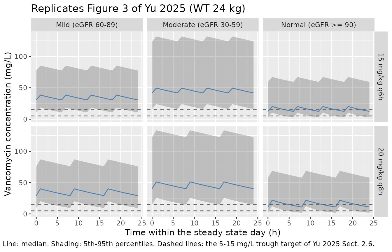
The qualitative findings of Fig. 3 reproduce: at 24 kg the normal-renal-function stratum sits inside the 5-15 mg/L trough target under both regimens, while both impairment strata exceed the upper limit, and the q6h regimen gives the higher trough of the two. The magnitudes in the impaired strata do not match Table 4; that is dissected below.
Clearance is a less-than-proportional function of eGFR
Yu 2025’s Key Points name body weight and glomerular filtration rate as the two important covariates on clearance. The eGFR exponent 0.812 being below 1 is what makes the renal effect less than proportional.
egfr_grid <- seq(30, 261, by = 1)
tibble::tibble(
  CRCL = egfr_grid,
  `Yu 2025 (exponent 0.812)` = 8.22 * (24 / 70)^0.75 * (egfr_grid / 173.42)^0.812,
  `Proportional (exponent 1)` = 8.22 * (24 / 70)^0.75 * (egfr_grid / 173.42)
) |>
  tidyr::pivot_longer(-CRCL, names_to = "Scaling", values_to = "cl") |>
  ggplot(aes(CRCL, cl, linetype = Scaling)) +
  geom_line() +
  geom_vline(xintercept = 173.42, colour = "grey50") +
  labs(
    x = "Schwartz eGFR (mL/min/1.73 m^2)",
    y = "Clearance at WT 24 kg (L/h)",
    title = "Less-than-proportional eGFR effect on vancomycin clearance",
    caption = "Vertical line: the 173.42 mL/min/1.73 m^2 reference. Yu 2025 Table 3, Eq. 12."
  ) +
  theme(legend.position = "bottom")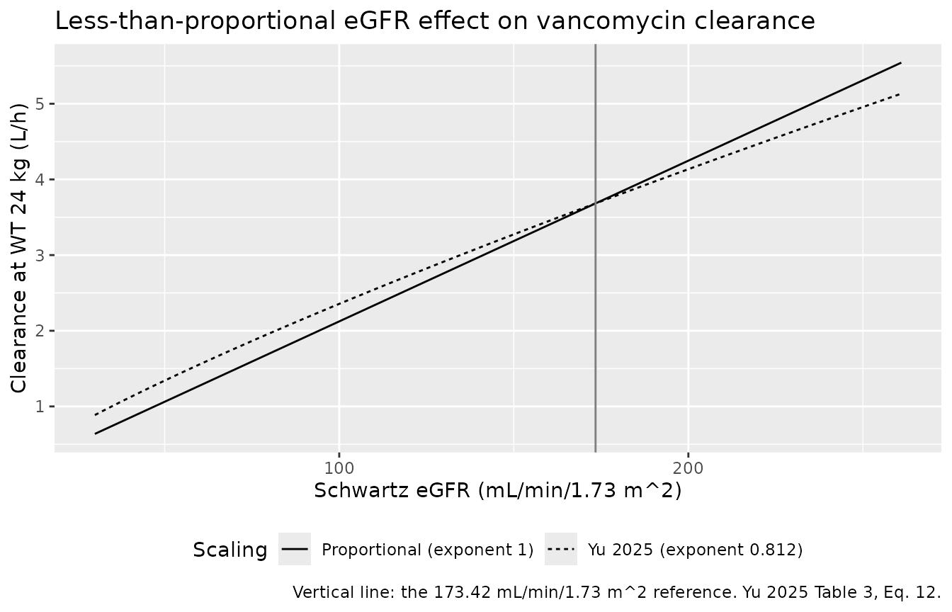
PKNCA validation
NCA is run over the steady-state 0-24 h window. The dose object
declares duration = 1 so PKNCA treats the records as
60-minute infusions rather than bolus doses.
sim_nca <- sim |>
  dplyr::filter(!is.na(Cc)) |>
  dplyr::select(id, time, Cc, treatment, renal)

# ss = 1 puts the steady-state trough on the time-zero record, so every subject
# already has a time-zero concentration; assert it rather than patching one in.
stopifnot(sum(sim_nca$time == 0) == 6L * n_per_arm)

dose_df <- events |>
  dplyr::filter(evid == 1) |>
  dplyr::select(id, time, amt, treatment, renal)

conc_obj <- PKNCA::PKNCAconc(
  sim_nca, Cc ~ time | treatment + renal + id,
  concu = "mg/L", timeu = "h"
)
dose_obj <- PKNCA::PKNCAdose(
  dose_df, amt ~ time | treatment + renal + id,
  doseu = "mg", duration = 1
)

intervals <- data.frame(
  start = 0, end = 24,
  auclast = TRUE, cmax = TRUE, cmin = TRUE, cav = TRUE
)

nca_res <- suppressWarnings(
  PKNCA::pk.nca(PKNCA::PKNCAdata(conc_obj, dose_obj, intervals = intervals))
)

nca <- as.data.frame(nca_res$result) |>
  dplyr::filter(start == 0, end == 24) |>
  dplyr::select(id, treatment, renal, PPTESTCD, PPORRES)

stopifnot(dplyr::n_distinct(nca$id) == 6L * n_per_arm)
Gate 1 - PKNCA AUC24 equals the analytic
Dose24 / CL
For a linear one-compartment model at steady state, AUC over a full day is exactly the daily dose divided by clearance, independent of the dosing interval and of the infusion duration. Reproducing that from the ODE solution end to end validates the structural model, the steady-state setup, and the NCA at once.
auc24 <- nca |>
  dplyr::filter(PPTESTCD == "auclast") |>
  dplyr::select(id, treatment, renal, AUC24 = PPORRES)

analytic <- events |>
  dplyr::filter(evid == 1) |>
  dplyr::group_by(id) |>
  dplyr::summarise(dose_24h = sum(amt), .groups = "drop") |>
  dplyr::left_join(
    sim |> dplyr::group_by(id) |> dplyr::summarise(cl = dplyr::first(cl), .groups = "drop"),
    by = "id"
  ) |>
  dplyr::mutate(AUC24_analytic = dose_24h / cl)

gate1 <- auc24 |>
  dplyr::left_join(analytic, by = "id") |>
  dplyr::mutate(rel_err = AUC24 / AUC24_analytic - 1)

stopifnot(nrow(gate1) == 6L * n_per_arm, !anyNA(gate1$rel_err))
max_rel_err <- max(abs(gate1$rel_err))
max_rel_err
#> [1] 3.037444e-05
stopifnot(max_rel_err < 1e-3)
The worst per-subject discrepancy across all 1200 subject-arms is 0.0030%, which is the residual lin-up/log-down interpolation error of the observation grid, not a model discrepancy.
Gate 2 - the two regimens deliver identical AUC24, subject by subject
20 mg/kg q8h and 15 mg/kg q6h are both 60 mg/kg/day. Because the model is linear and both arms are the same cohort, every subject’s AUC24 must be identical between the two regimens - not merely similar in distribution. This is the strongest available guard on the structural model and the steady-state setup, because it would fail if either arm’s dosing were mis-specified.
gate2 <- auc24 |>
  dplyr::left_join(
    events |> dplyr::distinct(id, subject), by = "id"
  ) |>
  dplyr::select(subject, treatment, AUC24) |>
  tidyr::pivot_wider(names_from = treatment, values_from = AUC24) |>
  dplyr::mutate(rel_diff = `15 mg/kg q6h` / `20 mg/kg q8h` - 1)

stopifnot(nrow(gate2) == 3L * n_per_arm, !anyNA(gate2$rel_diff))
max_auc_diff <- max(abs(gate2$rel_diff))
max_auc_diff
#> [1] 8.176809e-07
stopifnot(max_auc_diff < 1e-3)
Gate 3 - PKNCA cmin is the steady-state trough
At steady state every trough within the day is the same, so the
cmin PKNCA returns over 0-24 h must equal the concentration
on the ss = 1 time-zero record. This gate ties the NCA
summary used in the Table 4 comparison below back to the raw solve.
trough_ss <- sim |>
  dplyr::filter(time == 0) |>
  dplyr::select(id, subject, treatment, renal, trough_solve = Cc)

gate3 <- nca |>
  dplyr::filter(PPTESTCD == "cmin") |>
  dplyr::select(id, cmin = PPORRES) |>
  dplyr::left_join(trough_ss, by = "id") |>
  dplyr::mutate(rel_err = cmin / trough_solve - 1)

stopifnot(nrow(gate3) == 6L * n_per_arm, !anyNA(gate3$rel_err))
max_cmin_err <- max(abs(gate3$rel_err))
max_cmin_err
#> [1] 2.421839e-10
stopifnot(max_cmin_err < 1e-8)
Gate 4 - the simulated median trough is the typical-value trough
The trough is a monotone decreasing function of clearance, and
eta has median zero, so the median of the simulated cohort
must converge to the typical-value prediction at the stratum’s median
eGFR. This checks that the IIV was encoded on the intended parameter and
on the intended scale: an omega on the wrong scale would
not move the median, but an eta attached to the wrong
parameter or a mis-signed exponent would.
typical_trough <- function(CRCL, mg_per_kg, tau) {
  ev <- rxode2::et(amt = mg_per_kg * 24, ii = tau, ss = 1, dur = 1, cmt = "central") |>
    rxode2::et(0, cmt = "central")
  out <- rxode2::rxSolve(
    mod, ev, params = c(WT = 24, CRCL = CRCL, etalcl = 0),
    omega = NA, returnType = "data.frame",
    # steady-state searches for long-half-life subjects exceed the default step budget
    maxsteps = 1e6
  )
  out$Cc[out$time == 0][1]
}

gate4 <- trough_ss |>
  dplyr::group_by(treatment, renal) |>
  dplyr::summarise(sim_median = median(trough_solve), .groups = "drop") |>
  dplyr::left_join(
    base_cohort |>
      dplyr::group_by(renal) |>
      dplyr::summarise(egfr_median = median(CRCL), .groups = "drop"),
    by = "renal"
  ) |>
  dplyr::left_join(regimens |> dplyr::select(treatment, mg_per_kg, tau), by = "treatment") |>
  dplyr::rowwise() |>
  dplyr::mutate(typical = typical_trough(egfr_median, mg_per_kg, tau)) |>
  dplyr::ungroup() |>
  dplyr::mutate(rel_diff = sim_median / typical - 1)

stopifnot(nrow(gate4) == 6L, !anyNA(gate4$rel_diff))
max_median_diff <- max(abs(gate4$rel_diff))
max_median_diff
#> [1] 0.09303314
# The tolerance is set by Monte Carlo noise, not by model error: the standard
# error of a log-normal median with omega = 0.565 and n = 200 is about 4.5%, so
# the worst of six arms is expected around 2 SE. The seed is fixed, so the
# realized value below is deterministic.
stopifnot(max_median_diff < 0.10)

gate4 |>
  dplyr::transmute(
    Regimen = treatment, `Renal stratum` = renal,
    `Stratum median eGFR` = round(egfr_median, 1),
    `Simulated median trough (mg/L)` = round(sim_median, 2),
    `Typical-value trough (mg/L)` = round(typical, 2),
    `% diff` = round(100 * rel_diff, 1)
  ) |>
  knitr::kable(
    caption = paste("Gate 4: the Monte Carlo median trough converges to the",
                    "typical-value prediction at each stratum's median eGFR.")
)| Regimen | Renal stratum | Stratum median eGFR | Simulated median trough (mg/L) | Typical-value trough (mg/L) | % diff |
|---|---|---|---|---|---|
| 15 mg/kg q6h | Mild (eGFR 60-89) | 75.8 | 30.66 | 28.16 | 8.9 |
| 15 mg/kg q6h | Moderate (eGFR 30-59) | 45.2 | 41.74 | 44.80 | -6.8 |
| 15 mg/kg q6h | Normal (eGFR >= 90) | 172.7 | 12.37 | 12.73 | -2.9 |
| 20 mg/kg q8h | Mild (eGFR 60-89) | 75.8 | 29.24 | 26.75 | 9.3 |
| 20 mg/kg q8h | Moderate (eGFR 30-59) | 45.2 | 40.29 | 43.34 | -7.0 |
| 20 mg/kg q8h | Normal (eGFR >= 90) | 172.7 | 11.10 | 11.46 | -3.1 |
Comparison against the published Table 4 troughs
reference_t4 <- tibble::tribble(
  ~treatment,      ~renal,                   ~cmin,
  "20 mg/kg q8h",  "Normal (eGFR >= 90)",    10.75,
  "20 mg/kg q8h",  "Mild (eGFR 60-89)",      19.35,
  "20 mg/kg q8h",  "Moderate (eGFR 30-59)",  29.87,
  "15 mg/kg q6h",  "Normal (eGFR >= 90)",    12.08,
  "15 mg/kg q6h",  "Mild (eGFR 60-89)",      22.16,
  "15 mg/kg q6h",  "Moderate (eGFR 30-59)",  32.24
)

simulated_t4 <- nca |>
  dplyr::filter(PPTESTCD == "cmin") |>
  dplyr::select(treatment, renal, PPTESTCD, PPORRES)

t4_table <- nlmixr2lib::ncaComparisonTable(
  simulated_t4, reference_t4,
  by     = c("treatment", "renal"),
  params = "cmin",
  units  = c(cmin = "mg/L")
)

knitr::kable(
  t4_table,
  caption = paste("Simulated versus Yu 2025 Table 4 median steady-state trough,",
                  "WT 24 kg. Simulated values are cohort medians.")
)| NCA parameter | treatment | renal | Reference | Simulated | % diff |
|---|---|---|---|---|---|
| Cmin (mg/L) | 20 mg/kg q8h | Normal (eGFR >= 90) | 10.8 | 11.1 | +3.3% |
| Cmin (mg/L) | 20 mg/kg q8h | Mild (eGFR 60-89) | 19.4 | 29.2 | +51.1%* |
| Cmin (mg/L) | 20 mg/kg q8h | Moderate (eGFR 30-59) | 29.9 | 40.3 | +34.9%* |
| Cmin (mg/L) | 15 mg/kg q6h | Normal (eGFR >= 90) | 12.1 | 12.4 | +2.4% |
| Cmin (mg/L) | 15 mg/kg q6h | Mild (eGFR 60-89) | 22.2 | 30.7 | +38.3%* |
| Cmin (mg/L) | 15 mg/kg q6h | Moderate (eGFR 30-59) | 32.2 | 41.7 | +29.5%* |
attr(t4_table, "footnote")
#> [1] "* differs from reference by more than ±20%."
The normal-renal-function stratum reproduces within a few percent under both regimens. Both impairment strata are over-predicted, by 30-51%.
Table 4 does not follow from Eq. 12 for the impaired strata
The mismatch is not an artifact of the eGFR values chosen above. Inverting the model - asking which eGFR would have to be assumed to reproduce each published median - shows that the normal stratum’s implied eGFR lands inside its stated band while both impairment strata’s implied values land above theirs.
implied_egfr <- function(target, mg_per_kg, tau) {
  uniroot(function(g) typical_trough(g, mg_per_kg, tau) - target, c(10, 600))$root
}

implied <- reference_t4 |>
  dplyr::left_join(regimens |> dplyr::select(treatment, mg_per_kg, tau), by = "treatment") |>
  dplyr::left_join(strata, by = "renal") |>
  dplyr::rowwise() |>
  dplyr::mutate(egfr_implied = implied_egfr(cmin, mg_per_kg, tau)) |>
  dplyr::ungroup() |>
  dplyr::mutate(
    verdict = dplyr::case_when(
      egfr_implied > egfr_hi ~ "above band",
      egfr_implied < egfr_lo ~ "below band",
      TRUE                   ~ "inside band"
    )
  )

# The normal stratum reconciles; both impairment strata do not, and both fail in
# the same direction. Asserting the direction turns the finding into a guard: a
# future change to the covariate exponent or the reference eGFR would break it.
stopifnot(
  implied$verdict[implied$renal == "Normal (eGFR >= 90)"] == "inside band",
  implied$verdict[implied$renal != "Normal (eGFR >= 90)"] == "above band"
)

implied |>
  dplyr::transmute(
    Regimen = treatment, `Renal stratum` = renal,
    `Published median trough (mg/L)` = cmin,
    `Stated eGFR band` = sprintf("%g-%g", egfr_lo, egfr_hi),
    `Implied eGFR` = round(egfr_implied, 1),
    Verdict = verdict
  ) |>
  knitr::kable(
    caption = paste("eGFR that Eq. 12 would need in order to reproduce each",
                    "Yu 2025 Table 4 median trough at WT 24 kg.")
)| Regimen | Renal stratum | Published median trough (mg/L) | Stated eGFR band | Implied eGFR | Verdict |
|---|---|---|---|---|---|
| 20 mg/kg q8h | Normal (eGFR >= 90) | 10.75 | 90-260.82 | 182.8 | inside band |
| 20 mg/kg q8h | Mild (eGFR 60-89) | 19.35 | 60-89 | 105.4 | above band |
| 20 mg/kg q8h | Moderate (eGFR 30-59) | 29.87 | 30-59 | 67.5 | above band |
| 15 mg/kg q6h | Normal (eGFR >= 90) | 12.08 | 90-260.82 | 181.7 | inside band |
| 15 mg/kg q6h | Mild (eGFR 60-89) | 22.16 | 60-89 | 98.1 | above band |
| 15 mg/kg q6h | Moderate (eGFR 30-59) | 32.24 | 30-59 | 65.3 | above band |
Table 4 is internally consistent with the rest of the paper: its medians reproduce the fold-increases quoted in Yu 2025 Sect. 4 (mild and moderate 0.8- and 1.78-fold above normal at q8h; 0.83- and 1.67-fold at q6h) exactly to the printed precision.
fold <- reference_t4 |>
  dplyr::group_by(treatment) |>
  dplyr::mutate(fold = cmin / cmin[renal == "Normal (eGFR >= 90)"] - 1) |>
  dplyr::ungroup() |>
  dplyr::filter(renal != "Normal (eGFR >= 90)")

published_fold <- c(0.80, 1.78, 0.83, 1.67)  # Yu 2025 Sect. 4, in the order below
stopifnot(max(abs(round(fold$fold, 2) - published_fold)) < 1e-8)

fold |>
  dplyr::transmute(
    Regimen = treatment, `Renal stratum` = renal,
    `Fold increase vs normal (from Table 4)` = round(fold, 3),
    `Quoted in Yu 2025 Sect. 4` = published_fold
  ) |>
knitr::kable(caption = "Table 4 is internally consistent with the Sect. 4 narrative.")| Regimen | Renal stratum | Fold increase vs normal (from Table 4) | Quoted in Yu 2025 Sect. 4 |
|---|---|---|---|
| 20 mg/kg q8h | Mild (eGFR 60-89) | 0.800 | 0.80 |
| 20 mg/kg q8h | Moderate (eGFR 30-59) | 1.779 | 1.78 |
| 15 mg/kg q6h | Mild (eGFR 60-89) | 0.834 | 0.83 |
| 15 mg/kg q6h | Moderate (eGFR 30-59) | 1.669 | 1.67 |
So the discrepancy is between Table 4 and Eq. 12, not inside Table 4. Solving for the eGFR exponent that would reproduce Table 4’s renal ratios at the stratum midpoints localizes it to that one parameter.
typical_trough_exp <- function(CRCL, mg_per_kg, tau, e_crcl) {
  ev <- rxode2::et(amt = mg_per_kg * 24, ii = tau, ss = 1, dur = 1, cmt = "central") |>
    rxode2::et(0, cmt = "central")
  out <- rxode2::rxSolve(
    mod, ev,
    params = c(WT = 24, CRCL = CRCL, etalcl = 0, e_crcl_cl = e_crcl),
    omega = NA, returnType = "data.frame",
    # steady-state searches for long-half-life subjects exceed the default step budget
    maxsteps = 1e6
  )
  out$Cc[out$time == 0][1]
}

midpoints <- c(`Normal (eGFR >= 90)` = (90 + 260.82) / 2,
               `Mild (eGFR 60-89)` = 74.5,
               `Moderate (eGFR 30-59)` = 44.5)

published_ratio <- function(stratum, treatment) {
  num <- reference_t4$cmin[reference_t4$renal == stratum &
                             reference_t4$treatment == treatment]
  den <- reference_t4$cmin[reference_t4$renal == "Normal (eGFR >= 90)" &
                             reference_t4$treatment == treatment]
  if (length(num) != 1L || length(den) != 1L) {
    stop("no unique Table 4 row for '", stratum, "' / '", treatment, "'")
  }
  num / den
}

exponent_for <- function(stratum, treatment, mg_per_kg, tau) {
  ratio_target <- published_ratio(stratum, treatment)
  uniroot(function(e) {
    typical_trough_exp(midpoints[[stratum]], mg_per_kg, tau, e) /
      typical_trough_exp(midpoints[["Normal (eGFR >= 90)"]], mg_per_kg, tau, e) -
      ratio_target
  }, c(0.05, 1.5))$root
}

impaired <- c("Mild (eGFR 60-89)", "Moderate (eGFR 30-59)")

implied_exponents <- regimens |>
  dplyr::select(treatment, mg_per_kg, tau) |>
  tidyr::expand_grid(Stratum = impaired) |>
  dplyr::rowwise() |>
  dplyr::mutate(
    Exponent = exponent_for(Stratum, treatment, mg_per_kg, tau)
  ) |>
  dplyr::ungroup() |>
  dplyr::select(Regimen = treatment, Stratum, Exponent)

# Every implied exponent sits well below the Table 3 estimate of 0.812, and at
# or below the lower bootstrap bound of 0.55.
stopifnot(all(implied_exponents$Exponent < 0.7))

implied_exponents |>
  dplyr::mutate(
    `Implied eGFR exponent` = round(Exponent, 3),
    `Yu 2025 Table 3 estimate` = 0.812,
    `Table 3 bootstrap 2.5-97.5th` = "0.55-1.06",
    Exponent = NULL
  ) |>
  knitr::kable(
    caption = paste("eGFR exponent that would reproduce the Table 4 renal ratios",
                    "at the stratum midpoints, versus the Table 3 estimate.")
)| Regimen | Stratum | Implied eGFR exponent | Yu 2025 Table 3 estimate | Table 3 bootstrap 2.5-97.5th |
|---|---|---|---|---|
| 20 mg/kg q8h | Mild (eGFR 60-89) | 0.528 | 0.812 | 0.55-1.06 |
| 20 mg/kg q8h | Moderate (eGFR 30-59) | 0.595 | 0.812 | 0.55-1.06 |
| 15 mg/kg q6h | Mild (eGFR 60-89) | 0.588 | 0.812 | 0.55-1.06 |
| 15 mg/kg q6h | Moderate (eGFR 30-59) | 0.609 | 0.812 | 0.55-1.06 |
Every implied exponent falls in the range 0.53-0.61, against the Table 3 estimate of 0.812 and its bootstrap interval of 0.55-1.06. In other words, Table 4’s renal-impairment effect is weaker than the model the paper reports. The most likely proximate cause is that the Monte Carlo drew covariates “using the initial dataset” (Sect. 2.6) rather than from the stated bands, so the effective eGFR in each impaired stratum was higher than the band implies - the cohort has only a handful of patients below 90 mL/min/1.73 m^2 (the Table 1 minimum is 31.9), and resampling a sparse tail will pull the stratum’s realized eGFR upward. The paper reports neither the per-stratum eGFR distribution nor the simulation dataset, so this cannot be settled from the published record.
Practical consequence. The packaged model is faithful to Yu 2025 Table 3 and Eqs. 12-13, which are the model. A user reproducing Table 4 or Fig. 3 for the renal-impairment strata should expect troughs 30-51% higher than the paper printed, and should treat the paper’s dose-reduction suggestions in Sect. 4 (15 mg/kg q12h and 10 mg/kg q8h for moderate impairment) as conservative relative to what Eq. 12 actually predicts.
Assumptions and deviations
- eGFR values within each renal stratum are assumed, not published. Yu 2025 Sect. 2.6 gives only the stratum bands and says 1000 virtual patients were simulated “using the initial dataset”. This vignette samples eGFR uniformly across each stated band (normal capped at the Table 1 maximum of 260.82). The choice was fixed before any comparison was run.
-
omega_CL= 56.5% is read as100 * omega, giving omega^2 = 0.319225. The paper labels the row with the symbolomega_CLand never defines a %CV transform. The alternative reading,%CV = sqrt(exp(omega^2) - 1) * 100, would give omega = 0.5265 instead of 0.565 - a 7% difference on the standard deviation that changes no conclusion here (it affects only the width of the simulated intervals, not any median). What is ruled out is the reported number being a variance: the asymptotic relative standard error of an estimated variance is at leastsqrt(2/N)= 14.1% for N = 100 subjects, whereas Table 3 reports an RSE of 10%, which is only attainable on the standard-deviation scale. - Table 4’s dispersion is labelled “IQR” but is far too wide for one. The normal-stratum q8h entry is 10.75 (2.12-30.28), a 14-fold span; a log-normal with omega = 0.565 has an IQR spanning only 2.2-fold. Fig. 3’s caption says its shading is the 5th-95th percentile, so the Table 4 parenthetical is probably a 5th-95th percentile range (or a range that also carries the residual error and the within-stratum eGFR spread). No assertion in this vignette depends on it, and only the medians are compared.
-
No residual error is applied in the simulations. Yu
2025 Sect. 2.6 states that interindividual variability
(
omega_CL) was included in the Monte Carlo and does not mention the residual error. SincepropSdwas fixed rather than estimated, and since the trough medians compared here are unaffected by a zero-median multiplicative error, leaving it out is the cleaner comparison. -
Steady state is imposed with
ss = 1rather than by burn-in. For the moderate-impairment stratum the terminal half-life at 24 kg reaches roughly 22 h, so a burn-in would need several simulated days to converge;ss = 1gives the exact steady state directly. - The model is used only within the paper’s stated range of validity. Yu 2025 Sect. 4 recommends against predicting concentrations above 20 mg/L, because the VPC’s 95th percentile was poorly reproduced from sparse high-concentration data. The impaired-stratum profiles above sit above that threshold and are shown to replicate Fig. 3, not as endorsed predictions.
-
The paper reports no NCA parameters. There is no
published Cmax, Tmax, AUC, or half-life to compare against, so the PKNCA
section validates against analytic identities
(
AUC24 = Dose24 / CL, dose linearity,cminequal to the steady-state trough) and the published Table 4 trough medians instead. - No supplement, erratum, or corrigendum was located. The article is open access with no supplementary material; a search of the journal landing page and PubMed found no correction notice as of the extraction date.