Antisecretory drugs, intragastric pH and erosive esophagitis healing MBMA (Howden 2025)
Source:vignettes/articles/Howden_2025_antisecretory_mbma.Rmd
Howden_2025_antisecretory_mbma.RmdModel and source
- Citation: Howden CW, Scarpignato C, Vaezi MF, Jacob R, Wolle M, Hunt RH. Mathematical model of the relationship between pH holding time and erosive esophagitis healing rates. CPT Pharmacometrics Syst Pharmacol. 2025;14(1):28-35. doi:10.1002/psp4.13235
- Description: MBMA. Study-arm-level sigmoid Emax model on the logit scale linking the steady-state percentage of 24 h with intragastric pH > 4 (holding-time ratio, HTR) of an antisecretory regimen (histamine H2-receptor antagonist, proton pump inhibitor or potassium-competitive acid blocker) to the erosive esophagitis healing rate at week 4 or week 8, pooled from 82 pH-metry studies and 104 randomized healing trials (Howden 2025). Between-drug and between-treatment random effects are scaled by each arm’s standard error of the logit healing rate; the model simulates arm-level healing rates, not individual patients.
- Article: https://doi.org/10.1002/psp4.13235
Howden et al. (2025) pooled two literature datasets: healthy-volunteer 24 h intragastric pH-metry studies, summarised per drug and dose as the mean percentage of a day with intragastric pH > 4 (the pH > 4 holding-time ratio, HTR), and randomized erosive esophagitis healing trials, summarised per drug, dose and week as the pooled healing rate. Merged by regimen, the two datasets give one HTR and one healing rate (with its standard error) per arm and week. The final model is a sigmoid Emax function of HTR on the logit of the healing rate, with a separate HTR50 for week 4 and week 8, and two nested random effects (between drug and between treatment within drug) that are both scaled by the arm’s standard error.
The model simulates arm-level healing rates, not patients: each
simulated id is one hypothetical study arm.
Population
- 82 phase I pH-metry studies in healthy volunteers (4297 participants in 201 dose arms; pH recorded between days 5 and 8 of daily dosing).
- 104 phase II/III randomized erosive esophagitis healing trials
(43,417 patients in 196 treatment arms, intention-to-treat healing rates
at week 4 and/or week 8). The abstract gives 103 trials; the Results and
Figure 1 give
- Regimens: placebo; the H2-receptor antagonists (H2RA) famotidine, nizatidine and ranitidine; the proton pump inhibitors (PPI) esomeprazole, lansoprazole, omeprazole, pantoprazole, rabeprazole, azeloprazole, dexlansoprazole and ilaprazole; and the potassium-competitive acid blockers (P-CAB) tegoprazan and vonoprazan (Table 1).
- Adults (search restricted to participants >= 18 years); MEDLINE and Embase up to 31 March 2023.
The same information is available programmatically via
rxode2::rxode(readModelDb("Howden_2025_antisecretory_mbma"))$population.
Source trace
The model is given in full as a NONMEM $PRED block
(“Final Model Code”) in the paper’s supplement; the parameter values are
the final estimates of Supplementary Table S2. With HR the
healing rate of arm i of drug d:
with and likewise for BTV.
| Quantity | Model name | Value | Source |
|---|---|---|---|
| Placebo (HTR = 0) healing rate E0 | logite0 |
logit(12.3%) | Table S2 (RSE 68.9%) |
| Maximum healing rate Emax | logitemax |
logit(95.9%) | Table S2 (RSE 2.3%) |
| HTR50, week 8 | lec50_wk8 |
log(26.9%) | Table S2 (RSE 21.6%) |
| HTR50, week 4 | lec50_wk4 |
log(45.7%) | Table S2 (RSE 22.0%); code
IF(WEEK.EQ.1) TVEPH50 = THETA(7)
|
| HTR50 non-approval effect | e_trt_approved_ec50 |
-46.5% (applied when TRT_APPROVED = 0) |
Table S2 (RSE 4.5%); code IF(APPR.EQ.0)
|
| HTR50 P-CAB effect | e_trt_pcab_ec50 |
-30.8% | Table S2 (RSE 45.1%); code CLASS.EQ.5
|
| HTR50 H2RA effect | e_trt_h2ra_ec50 |
+41.3% | Table S2 (RSE 21.8%); code CLASS.EQ.3
|
| Shape gamma | lhill |
log(1.31) | Table S2 (RSE 33.5%) |
| Between-drug variability | bdv_pct |
8.1 (% above 50% at SE = 1) | Table S2 (RSE 27.8%) |
| Between-treatment variability | btv_pct |
6.86 (% above 50% at SE = 1) | Table S2 (RSE 25.8%) |
| BTV approval effect | e_trt_approved_btv |
+205% (applied when TRT_APPROVED = 1) |
Table S2 (RSE 48.7%); code IF(APPR.EQ.1), see
Assumptions |
| BTV H2RA effect | e_trt_h2ra_btv |
-71% | Table S2 (RSE 13.0%); code CLASS.EQ.3
|
| Drug random effect | eta_drug_mu |
variance 1, fixed |
$OMEGA (1 FIX), BDV_ = TVBDV_*ETA(1)
|
| Treatment random effect | addSd |
SD 1, fixed |
$SIGMA (1 FIX), BTV_ = TVBTV_*EPS(1)
|
| Arm SE scaling of both random effects | SE_ARM |
per record | code IPRED = MU + EEHR_SE*BDV_ + EEHR_SE*BTV_
|
| Logit link and Emax structure |
mu, logit_ee_healing
|
– | code MU = EEHR0_ + PH4**GAMMA*(...); Figure 2 |
Analysis dataset (Table 1)
The arms below carry Table 1’s pooled HTR and observed healing rates. The approval flags follow the Table 1 footnote (nizatidine, ranitidine 300 mg once daily, azeloprazole and ilaprazole not approved; pantoprazole 80 mg once daily also flagged). Tegoprazan, which is not approved in the US or the EU, is coded as not approved.
tab1 <- tibble::tribble(
  ~drug, ~regimen, ~class, ~htr, ~hr_wk4, ~hr_wk8, ~approved,
  "Placebo", "", "Placebo", 10.2, 18.1, 22.8, 1,
  "Famotidine", "20 mg b.i.d.", "H2RA", 34.5, 33.3, 56.6, 1,
  "Nizatidine", "150 mg b.i.d.", "H2RA", 18.1, 30.9, 40.3, 0,
  "Ranitidine", "150 mg q.i.d.", "H2RA", 38.0, 41.4, 63.6, 1,
  "Ranitidine", "300 mg OD", "H2RA", 36.7, 29.4, 53.3, 0,
  "Esomeprazole", "20 mg b.i.d.", "PPI", 73.9, NA, 83.6, 1,
  "Esomeprazole", "20 mg OD", "PPI", 56.5, NA, 85.7, 1,
  "Esomeprazole", "40 mg OD", "PPI", 65.2, 72.4, 85.6, 1,
  "Lansoprazole", "15 mg OD", "PPI", 43.3, 70.0, 77.2, 1,
  "Lansoprazole", "30 mg OD", "PPI", 55.6, 77.5, 86.5, 1,
  "Lansoprazole", "60 mg OD", "PPI", 55.2, 70.8, 83.9, 1,
  "Omeprazole", "10 mg OD", "PPI", 32.8, 55.8, NA, 1,
  "Omeprazole", "20 mg OD", "PPI", 51.3, 66.0, 80.9, 1,
  "Omeprazole", "40 mg OD", "PPI", 61.4, 66.6, 80.1, 1,
  "Pantoprazole", "10 mg OD", "PPI", 34.9, 42.0, 58.6, 1,
  "Pantoprazole", "20 mg OD", "PPI", 40.8, 66.9, 78.8, 1,
  "Pantoprazole", "40 mg b.i.d.", "PPI", 70.8, NA, 46.2, 1,
  "Pantoprazole", "40 mg OD", "PPI", 48.6, 68.9, 84.5, 1,
  "Pantoprazole", "80 mg OD", "PPI", 28.0, 66.3, 86.3, 0,
  "Rabeprazole", "10 mg b.i.d.", "PPI", 73.5, 85.4, 91.3, 1,
  "Rabeprazole", "10 mg OD", "PPI", 53.8, 89.7, 96.1, 1,
  "Rabeprazole", "20 mg OD", "PPI", 59.7, 70.9, 86.1, 1,
  "Rabeprazole", "40 mg OD", "PPI", 71.5, 50.0, 84.6, 1,
  "Azeloprazole", "10 mg OD", "PPI", 57.5, 89.6, 94.4, 0,
  "Azeloprazole", "20 mg OD", "PPI", 64.5, 89.7, 96.8, 0,
  "Azeloprazole", "40 mg OD", "PPI", 72.4, 92.1, 94.4, 0,
  "Dexlansoprazole", "60 mg OD", "PPI", 68.1, NA, 86.1, 1,
  "Dexlansoprazole", "90 mg OD", "PPI", 69.8, NA, 87.6, 1,
  "Ilaprazole", "10 mg OD", "PPI", 77.2, 77.4, 84.8, 0,
  "Tegoprazan", "100 mg OD", "P-CAB", 70.4, 90.2, 95.1, 0,
  "Tegoprazan", "50 mg OD", "P-CAB", 68.2, 87.0, 95.0, 0,
  "Vonoprazan", "10 mg OD", "P-CAB", 64.7, 86.7, 87.6, 1,
  "Vonoprazan", "20 mg OD", "P-CAB", 88.2, 91.0, 93.5, 1,
  "Vonoprazan", "40 mg OD", "P-CAB", 96.6, 89.0, 89.0, 1
)

arms <- tab1 |>
  pivot_longer(c(hr_wk4, hr_wk8), names_to = "wk", values_to = "hr_obs") |>
  filter(!is.na(hr_obs)) |>
  mutate(week = ifelse(wk == "hr_wk4", 4, 8)) |>
  select(-wk)

class_cov <- function(cls) {
  data.frame(
    TRT_H2RA = as.integer(cls == "H2RA"),
    TRT_PCAB = as.integer(cls == "P-CAB")
  )
}
Typical response and prediction interval (Figure 4)
Figure 4 of the paper is a visual predictive check of approved
regimens: the typical healing-rate curve per drug class and week, with
an 80% prediction interval for large studies (SE = 0.25, about 300
patients). The curves below are the model’s typical values
(zeroRe()); the shaded bands are the 10th and 90th
percentiles of 200 simulated arms per HTR grid point. The dots are Table
1’s observed approved-regimen healing rates.
# eta_drug_mu shifts the model() quantity mu rather than an ini() parameter,
# so rxode2 warns that it is not mu-referenced; the typical-value copy has no
# omega or sigma left, which rxode2 also reports on every solve. Both are
# expected here and are silenced so the article shows only real problems.
mod <- suppressWarnings(rxode2::rxode2(readModelDb("Howden_2025_antisecretory_mbma")))
mod_typ <- suppressWarnings(zeroRe(mod))
classes <- c("H2RA", "PPI", "P-CAB")
grid <- expand.grid(
  GASTRIC_PH4_TIME_PCT = seq(0, 100, by = 4),
  class = classes,
  week = c(4, 8),
  stringsAsFactors = FALSE
)
grid <- cbind(grid, class_cov(grid$class))
grid$TRT_APPROVED <- 1
grid$SE_ARM <- 0.25
grid$point <- seq_len(nrow(grid))

typ_ev <- grid |>
  mutate(id = point, time = week, evid = 0, amt = 0)
typ <- as.data.frame(suppressWarnings(rxSolve(mod_typ, typ_ev, keep = c("class", "week"))))
#> ℹ omega/sigma items treated as zero: 'eta_drug_mu'

n_rep <- 200
sim_ev <- grid[rep(seq_len(nrow(grid)), each = n_rep), ] |>
  mutate(id = seq_len(n()), time = week, evid = 0, amt = 0)
rxSetSeed(20250101)
sim <- as.data.frame(rxSolve(mod, sim_ev,
  keep = c("class", "week", "point"),
  returnType = "data.frame"
))
sim$hr_sim <- 100 * plogis(sim$sim)

band <- sim |>
  group_by(class, week, GASTRIC_PH4_TIME_PCT) |>
  summarise(
    lo = quantile(hr_sim, 0.1), hi = quantile(hr_sim, 0.9),
    .groups = "drop"
  )
obs_appr <- arms |>
  filter(approved == 1, class %in% classes)
ggplot() +
  geom_ribbon(
    data = band,
    aes(GASTRIC_PH4_TIME_PCT, ymin = lo, ymax = hi, fill = class), alpha = 0.2
  ) +
  geom_line(data = typ, aes(GASTRIC_PH4_TIME_PCT, ee_healing, colour = class)) +
  geom_point(data = obs_appr, aes(htr, hr_obs, colour = class)) +
  facet_wrap(~ paste("Week", week)) +
  scale_x_continuous(limits = c(0, 100)) +
  scale_y_continuous(limits = c(0, 100)) +
  labs(
    x = "Mean time with intragastric pH > 4 (% of 24 h)",
    y = "Erosive esophagitis healing rate (%)",
    colour = "Drug class", fill = "Drug class"
  ) +
  theme_bw()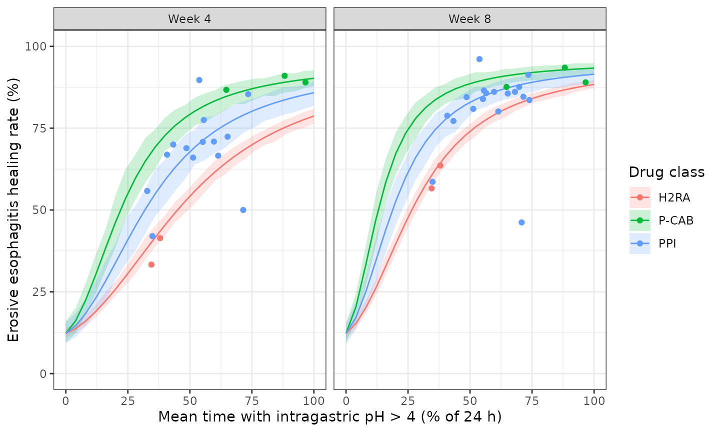
Replicates Figure 4 of Howden 2025: typical healing rate (line) and 80% prediction interval for SE = 0.25 studies (band) of approved regimens, with Table 1 approved-regimen observations (dots).
At HTR = 0 every curve starts at the placebo healing rate E0 = 12.3%, and at 100% HTR the week-8 PPI and P-CAB curves reach about 92-93%, as in Figure 4.
e0 <- typ |>
  filter(GASTRIC_PH4_TIME_PCT == 0, class == "PPI", week == 8)
w8_top <- typ |>
  filter(GASTRIC_PH4_TIME_PCT == 100, week == 8) |>
  select(class, ee_healing)
w8_top
#>   class ee_healing
#> 1  H2RA   88.37062
#> 2   PPI   91.49248
#> 3 P-CAB   93.35800
stopifnot(
  abs(e0$ee_healing - 12.3) < 1,
  all(w8_top$ee_healing[w8_top$class != "H2RA"] > 90),
  all(w8_top$ee_healing[w8_top$class != "H2RA"] < 95.9)
)
Required pH > 4 holding time (Table S3)
Table S3 lists the hours per day of pH > 4 that the typical approved regimen of each class needs to reach a healing rate of 80%, 85% or 90%. Inverting the Emax model for HTR gives
“not achievable” when the result exceeds 100%. The closed form is checked against the model by solving it at the required HTR, which must return the target healing rate.
th <- as.list(rxode2::rxode(mod)$theta)
ec50_class <- function(cls, week) {
  base <- exp(if (week == 4) th$lec50_wk4 else th$lec50_wk8)
  base * (1 + th$e_trt_pcab_ec50 * (cls == "P-CAB")) *
    (1 + th$e_trt_h2ra_ec50 * (cls == "H2RA"))
}
req <- expand.grid(
  target = c(80, 85, 90), class = classes, week = c(4, 8),
  stringsAsFactors = FALSE
)
req$f <- (qlogis(req$target / 100) - th$logite0) / (th$logitemax - th$logite0)
req$htr_req <- mapply(ec50_class, req$class, req$week) *
  (req$f / (1 - req$f))^(1 / exp(th$lhill))
req$hours <- ifelse(req$htr_req > 100, NA, req$htr_req / 100 * 24)

# Self-consistency: the model solved at the required HTR returns the target.
chk_ev <- req |>
  filter(!is.na(hours)) |>
  mutate(
    id = seq_len(n()), time = week, evid = 0, amt = 0,
    GASTRIC_PH4_TIME_PCT = htr_req, TRT_APPROVED = 1, SE_ARM = 0.5
  )
chk_ev <- cbind(chk_ev, class_cov(chk_ev$class))
chk <- as.data.frame(suppressWarnings(rxSolve(mod_typ, chk_ev, keep = "target")))
#> ℹ omega/sigma items treated as zero: 'eta_drug_mu'
stopifnot(max(abs(chk$ee_healing - chk$target)) < 1e-6)

paper_hours <- tibble::tribble(
  ~target, ~class, ~week, ~paper,
  80, "H2RA", 4, NA, 80, "H2RA", 8, 15.3,
  80, "PPI", 4, 17.7, 80, "PPI", 8, 10.5,
  80, "P-CAB", 4, 12.0, 80, "P-CAB", 8, 7.2,
  85, "H2RA", 4, NA, 85, "H2RA", 8, 19.5,
  85, "PPI", 4, 22.6, 85, "PPI", 8, 13.5,
  85, "P-CAB", 4, 15.4, 85, "P-CAB", 8, 9.2,
  90, "H2RA", 4, NA, 90, "H2RA", 8, NA,
  90, "PPI", 4, NA, 90, "PPI", 8, 20.5,
  90, "P-CAB", 4, 23.4, 90, "P-CAB", 8, 14.0
)
hours_cmp <- req |>
  select(target, class, week, hours) |>
  left_join(paper_hours, by = c("target", "class", "week")) |>
  mutate(pct_diff = 100 * (hours - paper) / paper) |>
  arrange(target, class, week)
hours_cmp |>
  mutate(hours = round(hours, 1), pct_diff = round(pct_diff, 1)) |>
  rename(
    "Target healing rate (%)" = target, "Drug class" = class, "Week" = week,
    "Required h/day (model)" = hours, "Required h/day (Table S3)" = paper,
    "Difference (%)" = pct_diff
  ) |>
knitr::kable()| Target healing rate (%) | Drug class | Week | Required h/day (model) | Required h/day (Table S3) | Difference (%) |
|---|---|---|---|---|---|
| 80 | H2RA | 4 | NA | NA | NA |
| 80 | H2RA | 8 | 14.9 | 15.3 | -2.8 |
| 80 | P-CAB | 4 | 12.4 | 12.0 | 3.1 |
| 80 | P-CAB | 8 | 7.3 | 7.2 | 1.2 |
| 80 | PPI | 4 | 17.9 | 17.7 | 1.0 |
| 80 | PPI | 8 | 10.5 | 10.5 | 0.3 |
| 85 | H2RA | 4 | NA | NA | NA |
| 85 | H2RA | 8 | 19.0 | 19.5 | -2.7 |
| 85 | P-CAB | 4 | 15.8 | 15.4 | 2.5 |
| 85 | P-CAB | 8 | 9.3 | 9.2 | 1.0 |
| 85 | PPI | 4 | 22.8 | 22.6 | 0.9 |
| 85 | PPI | 8 | 13.4 | 13.5 | -0.6 |
| 90 | H2RA | 4 | NA | NA | NA |
| 90 | H2RA | 8 | NA | NA | NA |
| 90 | P-CAB | 4 | 23.3 | 23.4 | -0.2 |
| 90 | P-CAB | 8 | 13.7 | 14.0 | -1.9 |
| 90 | PPI | 4 | NA | NA | NA |
| 90 | PPI | 8 | 19.9 | 20.5 | -3.1 |
Every entry the paper marks “not achievable” is also above 100% HTR here, and the achievable entries agree within a few percent (rounding of the Table S2 estimates, notably gamma = 1.31, moves the inverted HTR by that much).
Probability of achieving a target healing rate (Table S3, Figure 6)
The paper simulated each drug class at its aggregated HTR levels for
studies with SE = 0.5 (about 100 patients) and reported the fraction of
simulated studies reaching a healing rate of at least 80%, 85% or 90%.
Only approved regimens enter the simulations. Because both random
effects are normal on the logit scale, the probability for one arm is
exact:
1 - pnorm((logit(p) - mu) / (SE_ARM * sqrt(sdDrug^2 + sdTrt^2))),
using the model’s own mu, sdDrug and
sdTrt. The class probability averages this over the class’s
approved arms observed at that week. The Table S3 “average time
observed” (7.5 h H2RA, 13.7 h PPI, 20.0 h P-CAB) guides the arm sets:
the PPI value is the mean of the approved PPI regimens of Table 1, and
the P-CAB value is the mean of the three vonoprazan regimens, which
excludes tegoprazan. No H2RA subset gives 7.5 h exactly (the two
approved regimens give 8.7 h, adding nizatidine 7.3 h, all four 7.6 h);
the H2RA probabilities are zero for every choice.
sim_arms <- arms |>
  filter(class %in% classes, approved == 1)
sim_arms |>
  distinct(class, drug, regimen, htr) |>
  group_by(class) |>
  summarise(mean_hours = round(mean(htr) / 100 * 24, 1)) |>
  rename("Drug class" = class, "Mean pH > 4 time (h/day)" = mean_hours) |>
knitr::kable()| Drug class | Mean pH > 4 time (h/day) |
|---|---|
| H2RA | 8.7 |
| P-CAB | 20.0 |
| PPI | 13.7 |
prob_ev <- sim_arms |>
  mutate(
    id = seq_len(n()), time = week, evid = 0, amt = 0,
    GASTRIC_PH4_TIME_PCT = htr, TRT_APPROVED = 1, SE_ARM = 0.5
  )
prob_ev <- cbind(prob_ev, class_cov(prob_ev$class))
prob_typ <- as.data.frame(suppressWarnings(rxSolve(mod_typ, prob_ev,
  keep = "class"
)))
#> ℹ omega/sigma items treated as zero: 'eta_drug_mu'

prob_model <- prob_typ |>
  crossing(target = c(80, 85, 90)) |>
  mutate(
    p_arm = 1 - pnorm((qlogis(target / 100) - mu) /
      (SE_ARM * sqrt(sdDrug^2 + sdTrt^2)))
  ) |>
  group_by(target, class, week = time) |>
  summarise(model = 100 * mean(p_arm), .groups = "drop")

# Stochastic cross-check: 200 simulated studies per arm.
n_rep <- 200
mc_ev <- prob_ev[rep(seq_len(nrow(prob_ev)), each = n_rep), ] |>
  mutate(id = seq_len(n()))
rxSetSeed(20250102)
mc <- as.data.frame(rxSolve(mod, mc_ev, keep = "class", returnType = "data.frame"))
mc$hr_sim <- 100 * plogis(mc$sim)
prob_mc <- mc |>
  crossing(target = c(80, 85, 90)) |>
  group_by(target, class, week = time) |>
  summarise(simulated = 100 * mean(hr_sim >= target), .groups = "drop")

paper_prob <- tibble::tribble(
  ~target, ~class, ~week, ~paper,
  80, "H2RA", 4, 0.0, 80, "H2RA", 8, 0.0,
  80, "PPI", 4, 19.7, 80, "PPI", 8, 75.5,
  80, "P-CAB", 4, 90.0, 80, "P-CAB", 8, 99.2,
  85, "H2RA", 4, 0.0, 85, "H2RA", 8, 0.0,
  85, "PPI", 4, 6.1, 85, "PPI", 8, 50.0,
  85, "P-CAB", 4, 70.9, 85, "P-CAB", 8, 95.4,
  90, "H2RA", 4, 0.0, 90, "H2RA", 8, 0.0,
  90, "PPI", 4, 0.6, 90, "PPI", 8, 17.3,
  90, "P-CAB", 4, 35.1, 90, "P-CAB", 8, 74.1
)
prob_cmp <- prob_model |>
  left_join(prob_mc, by = c("target", "class", "week")) |>
  left_join(paper_prob, by = c("target", "class", "week")) |>
  mutate(diff = model - paper) |>
  arrange(target, class, week)
prob_cmp |>
  mutate(across(c(model, simulated, diff), \(x) round(x, 1))) |>
  rename(
    "Target healing rate (%)" = target, "Drug class" = class, "Week" = week,
    "P(success) exact (%)" = model, "P(success) simulated (%)" = simulated,
    "P(success) Table S3 (%)" = paper, "Exact minus paper (points)" = diff
  ) |>
knitr::kable()| Target healing rate (%) | Drug class | Week | P(success) exact (%) | P(success) simulated (%) | P(success) Table S3 (%) | Exact minus paper (points) |
|---|---|---|---|---|---|---|
| 80 | H2RA | 4 | 0.0 | 0.0 | 0.0 | 0.0 |
| 80 | H2RA | 8 | 0.0 | 0.0 | 0.0 | 0.0 |
| 80 | P-CAB | 4 | 89.0 | 90.8 | 90.0 | -1.0 |
| 80 | P-CAB | 8 | 99.1 | 99.0 | 99.2 | -0.1 |
| 80 | PPI | 4 | 16.7 | 15.4 | 19.7 | -3.0 |
| 80 | PPI | 8 | 75.6 | 76.1 | 75.5 | 0.1 |
| 85 | H2RA | 4 | 0.0 | 0.0 | 0.0 | 0.0 |
| 85 | H2RA | 8 | 0.0 | 0.0 | 0.0 | 0.0 |
| 85 | P-CAB | 4 | 70.4 | 72.5 | 70.9 | -0.5 |
| 85 | P-CAB | 8 | 94.8 | 95.5 | 95.4 | -0.6 |
| 85 | PPI | 4 | 5.5 | 5.2 | 6.1 | -0.6 |
| 85 | PPI | 8 | 52.3 | 52.4 | 50.0 | 2.3 |
| 90 | H2RA | 4 | 0.0 | 0.0 | 0.0 | 0.0 |
| 90 | H2RA | 8 | 0.0 | 0.0 | 0.0 | 0.0 |
| 90 | P-CAB | 4 | 34.8 | 38.0 | 35.1 | -0.3 |
| 90 | P-CAB | 8 | 74.0 | 73.2 | 74.1 | -0.1 |
| 90 | PPI | 4 | 0.6 | 0.6 | 0.6 | 0.0 |
| 90 | PPI | 8 | 20.4 | 20.3 | 17.3 | 3.1 |
ggplot(prob_cmp, aes(paste("Week", week), model, fill = class)) +
  geom_col(position = position_dodge(0.9)) +
  geom_point(aes(y = paper),
    position = position_dodge(0.9), shape = 4, size = 2.5
  ) +
  facet_wrap(~ paste0("Minimum healing rate ", target, "%")) +
  labs(x = NULL, y = "Probability of achieving healing rate (%)", fill = "Drug class") +
  theme_bw()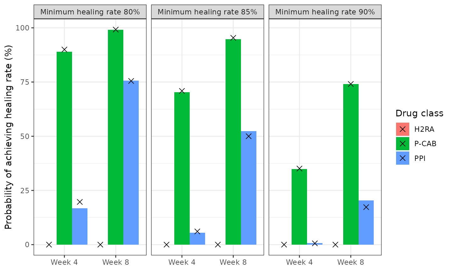
Replicates Figure 6 of Howden 2025: probability of a study (SE = 0.5) achieving at least the target healing rate, by drug class and week. Bars are the model; crosses are Table S3.
The P-CAB probabilities reproduce Table S3 to within about one percentage point and the H2RA probabilities are zero, as in the paper. The PPI probabilities agree to within about three points; the paper does not list which PPI regimens it counted as approved, and the Table 1 approval footnotes, which are used here, reproduce its 13.7 h average but not every probability exactly.
pc <- split(prob_cmp, prob_cmp$class)
stopifnot(
  max(abs(pc[["P-CAB"]]$diff)) < 1.5,
  max(pc[["H2RA"]]$model) < 0.5,
  max(abs(pc[["PPI"]]$diff)) < 4,
  # The Monte Carlo estimate agrees with the exact average (200 studies per
  # arm; the binomial SE of a pooled class probability is below 2 points).
  max(abs(prob_cmp$simulated - prob_cmp$model)) < 6
)
NCA
No NCA is performed: the model has no drug concentrations, doses or time course. Its input is a regimen-level pharmacodynamic summary (HTR) and its output is an arm-level healing rate at week 4 or week 8, so the validation above uses the paper’s own tabulated predictions instead of PKNCA.
Assumptions and deviations
-
Final estimates from Table S2, not the printed
$THETAblock. The$THETAblock of the supplement’s Final Model Code lists a different set of numbers (e.g. E0 10.32, EHTR50 week 8 24.74, BTV approval effect 165.4). Those are initial or earlier-run values; Table S2 is used throughout. The check above (required hours and probabilities of success) reproduces Table S3 with the Table S2 values. - E0 = 12.3%. The Results text gives the placebo healing rate as 10.6% (RSE 70%); Table S2 gives 12.3% (RSE 68.9%). The Table S2 value reproduces the Table S3 required holding times and the 12% intercept of Figure 4; 10.6% does not.
-
Direction of the BTV approval effect. Table S2
labels the +205% BTV effect “Non-approval effect”, and its footnote says
between-treatment variability was larger for non-approved treatments,
but the Final Model Code applies it when
APPR.EQ.1(approved). The code is followed: with it the simulated P-CAB week-8 probability of a >= 90% healing rate is 74% (Table S3: 74.1%), whereas applying the effect to non-approved regimens instead gives about 88%. In the model it therefore multiplies the between-treatment SD by 3.05 for approved regimens. -
Week as observation time. The NONMEM
WEEKflag is encoded from the observation time: records attime = 4(weeks) use the week-4 HTR50 and records attime = 8the week-8 value. The model is only defined at those two times. -
Between-drug random effect name.
eta_drug_muacts on the logit-scale predictionmu, which is amodel()quantity rather than anini()parameter, socheckModelConventions()reports that it has no matching fixed effect. The name records the grouping level (drug) and the quantity it shifts, as in the source. - Arm sets for the Table S3 simulations. The paper does not list the arms it simulated. Approved regimens per the Table 1 footnotes are used; tegoprazan is treated as not approved because it is not approved in the US or the EU, which is what the P-CAB 20.0 h average requires.
-
Placebo is not a drug class here. Placebo arms have
TRT_H2RA = 0andTRT_PCAB = 0, like PPI arms; the model distinguishes them only by their low HTR (10.2%).