Benzylpenicillin (Shah 2023)
Source:vignettes/articles/Shah_2023_benzylpenicillin.Rmd
Shah_2023_benzylpenicillin.RmdModel and source
- Citation: Shah RV, Kipper K, Baker EH, Barker CIS, Oldfield I, Philips BJ, Johnston A, Lipman J, Rhodes A, Basarab M, Sharland M, Almahdi S, Wake RM, Standing JF, Lonsdale DO (2023). Population Pharmacokinetic Study of Benzylpenicillin in Critically Unwell Adults. Antibiotics 12(4):643. doi:10.3390/antibiotics12040643.
- Description: Two-compartment intravenous population PK model for benzylpenicillin in critically unwell adults, with a priori allometric body-weight scaling on all disposition parameters and a serum-creatinine power effect on clearance.
- Article: https://doi.org/10.3390/antibiotics12040643
- Supplement (Tables S1 and S2): https://www.mdpi.com/article/10.3390/antibiotics12040643/s1
Shah and colleagues report the first full population pharmacokinetic analysis of benzylpenicillin in critically unwell adults, using data from the ABDose observational antibiotic study. The final model is a two-compartment intravenous disposition model with a priori allometric body-weight scaling on all four disposition parameters and a power effect of serum creatinine on clearance.
Population
Twelve adults admitted to the intensive care unit of St George’s Hospital, London, and prescribed intravenous benzylpenicillin contributed 80 plasma samples, of which 77 entered the analysis (Shah 2023, Section 2). Eight patients received 1.2 g four-hourly, two received 1.2 g six-hourly, and two received 2.4 g four-hourly. Sampling was opportunistic within a dosing interval (Table 3).
Baseline characteristics (Table 1): median age 57.7 years (IQR 44.3-63.2, range 25.7-71.7); 6 male and 6 female; median weight 70.0 kg (IQR 65.7-90.0, range 60.0-120.0); median height 172.0 cm; median BMI 26.1 kg/m^2; median serum creatinine 70 (IQR 52-103.5, range 34-486); median serum albumin 28 g/L; median APACHE II 14 points. Treated infection sources were lower respiratory tract infection (7), skin or soft-tissue infection / abscess (5), infective endocarditis (1) and sepsis of unknown source (1). Five patients received vasopressors. One patient received renal replacement therapy; only samples drawn after renal recovery and cessation of RRT were analysed. Three participants had acute kidney injury with serum creatinine ranging 176-486.
The same information is available programmatically from the model’s
population metadata:
str(readModelDb("Shah_2023_benzylpenicillin")()$population)
#> List of 17
#>  $ species       : chr "human"
#>  $ n_subjects    : num 12
#>  $ n_studies     : num 1
#>  $ n_samples     : num 77
#>  $ age_range     : chr "25.7-71.7 years"
#>  $ age_median    : chr "57.7 years"
#>  $ weight_range  : chr "60.0-120.0 kg"
#>  $ weight_median : chr "70.0 kg"
#>  $ height_range  : chr "150.0-188.0 cm"
#>  $ sex_female_pct: num 50
#>  $ race_ethnicity: Named num [1:5] 50 8.3 16.7 8.3 16.7
#>   ..- attr(*, "names")= chr [1:5] "White British" "White Irish" "Asian" "Caribbean" ...
#>  $ disease_state : chr "Critical illness requiring intensive care; treated infection sources were lower respiratory tract infection (7)"| __truncated__
#>  $ dose_range    : chr "1.2 g IV 4-hourly (8 patients), 1.2 g IV 6-hourly (2 patients), 2.4 g IV 4-hourly (2 patients)"
#>  $ regions       : chr "United Kingdom (single centre: St George's Hospital, London)"
#>  $ renal_function: chr "Serum creatinine median 70 umol/L (IQR 52-103.5, range 34-486); three participants had acute kidney injury. One"| __truncated__
#>  $ severity      : chr "APACHE II median 14 points (IQR 12.5-18, range 5-23); 5 patients on vasopressors; 1 intubated and ventilated, 3"| __truncated__
#>  $ notes         : chr "Sub-study of the ABDose observational antibiotic PK/PD study (REC 14/LO/1999). Baseline demographics: Shah 2023"| __truncated__
Source trace
The per-parameter origin is recorded as an in-file comment next to
each ini() entry in
inst/modeldb/specificDrugs/Shah_2023_benzylpenicillin.R.
The table below collects them in one place for review.
| Equation / parameter | Value | Source location |
|---|---|---|
lcl (CL) |
23.1 L/h/70 kg | Table 2, theta_CL (14% RSE); bootstrap median 24.0
(19.0-31.5) |
lvc (V1) |
15.1 L/70 kg | Table 2, theta_V1 (8% RSE); bootstrap median 14.4
(9.4-16.8) |
lq (Q) |
11.1 L/h/70 kg | Table 2, theta_Q (50% RSE); bootstrap median 11.4
(7.0-39.4) |
lvp (V2) |
9.8 L/70 kg | Table 2, theta_V2 (29% RSE); bootstrap median 10.5
(7.4-21.3) |
e_creat_cl |
-0.916 | Table 2, theta_CREAT (18% RSE); bootstrap median -0.97
(-1.26 to -0.67) |
e_wt_cl_q |
fixed 0.75 | Section 4: “clearance parameters were scaled to an allometric exponent of 0.75” |
e_wt_vc_vp |
fixed 1 | Section 4: “Compartment volumes were scaled with a fixed exponent of 1” |
etalcl |
42.0 %CV -> 0.16246 | Table 2, omega^2_1 CL (43% RSE);
omega^2 = log(CV^2 + 1)
|
etalvc |
22.6 %CV -> 0.04981 | Table 2, omega^2_2 V1 (42% RSE) |
etalvp |
20.5 %CV -> 0.04117 | Table 2, omega^2_3 V2 (60% RSE) |
| (no IIV on Q) | n/a | Section 2: “interindividual variability were added to all parameters other than Q, for which this parameter was found to be negligible” |
propSd |
sqrt(0.021) = 0.14491 | Table 2, sigma^2_1 (proportional), 47% RSE |
addSd |
sqrt(0.006) = 0.07746 | Table 2, sigma^2_2 (additive), 67% RSE |
| CL covariate equation | CL = theta_CL * exp(eta_1) * (Creatinine / 70)^theta_creat |
Equation (1) |
| Two-compartment IV structure | n/a | Section 2 (dOFV -104.4 vs one-compartment); Supplementary Table S1 runs 1-2 |
| Reference weight 70 kg | n/a | Table 2 (all thetas reported “/70 kg”) |
| Reference creatinine 70 | n/a | Equation (1) denominator; equals the Table 1 cohort median |
| Protein binding 60% (fu = 0.40) | n/a | Section 4: “Protein binding of 60% was assumed, with 40% remaining unbound and pharmacologically active” |
| Derived elimination half-life | 1.11 h | Table 2, “Derived parameters”; Section 3 states 67 min |
Virtual cohort
The original observed data are not publicly available (Shah 2023, Data Availability Statement). The simulations below use a virtual population whose covariate distributions approximate the published Table 1 demographics.
Shah 2023 simulated 10,000 patients with the linpk
package but does not state the covariate distributions used, so body
weight and serum creatinine are drawn here from log-normal distributions
matched to the Table 1 median and interquartile range and truncated to
the Table 1 full range. This assumption is recorded under “Assumptions
and deviations” below.
Five dosing regimens are simulated, matching Shah 2023 Section 2 and Supplementary Table S2:
- 1.2 g bolus four-hourly; (b) 2.4 g bolus four-hourly; (c) 1.2 g bolus followed by a 6 g continuous infusion over 24 h; (d) 7.2 g continuous infusion over 24 h; (e) 1.2 g extended infusion over 2 h, four-hourly.
set.seed(20230324)

n_per_arm <- 200  # per-arm cap; 200 is ample for a percentile-based VPC
obs_times <- seq(0, 24, by = 0.05)

# Log-normal parameters matched to the Table 1 medians and IQRs.
# sdlog = log(Q3 / Q1) / (2 * qnorm(0.75))
wt_meanlog    <- log(70)
wt_sdlog      <- log(90 / 65.7) / (2 * qnorm(0.75))
creat_meanlog <- log(70)
creat_sdlog   <- log(103.5 / 52) / (2 * qnorm(0.75))

draw_covariates <- function(n) {
  # Truncated to the Table 1 full ranges (WT 60-120 kg; CREAT 34-486).
  tibble(
    WT    = pmin(pmax(rlnorm(n, wt_meanlog, wt_sdlog), 60), 120),
    CREAT = pmin(pmax(rlnorm(n, creat_meanlog, creat_sdlog), 34), 486)
  )
}

# `dose_spec` describes one regimen as a set of dose records. `rate = 0` is an
# instantaneous bolus; `rate > 0` (mg/h) is a zero-order infusion of duration
# amt / rate.
regimens <- list(
  list(label = "1.2 g bolus q4h",
       doses = tibble(time = seq(0, 20, by = 4), amt = 1200, rate = 0)),
  list(label = "2.4 g bolus q4h",
       doses = tibble(time = seq(0, 20, by = 4), amt = 2400, rate = 0)),
  list(label = "1.2 g bolus + 6 g CI/24 h",
       doses = tibble(time = c(0, 0), amt = c(1200, 6000), rate = c(0, 6000 / 24))),
  list(label = "7.2 g CI/24 h",
       doses = tibble(time = 0, amt = 7200, rate = 7200 / 24)),
  list(label = "1.2 g over 2 h q4h",
       doses = tibble(time = seq(0, 20, by = 4), amt = 1200, rate = 1200 / 2))
)

make_arm <- function(spec, n, id_offset) {
  covs <- draw_covariates(n) |>
    mutate(id = id_offset + seq_len(n), regimen = spec$label)

  dosing <- covs |>
    tidyr::crossing(spec$doses) |>
    mutate(evid = 1L, cmt = "central")

  obs <- covs |>
    tidyr::crossing(time = obs_times) |>
    mutate(amt = NA_real_, rate = 0, evid = 0L, cmt = "central")

  bind_rows(dosing, obs) |>
    arrange(id, time, desc(evid)) |>
    select(id, time, amt, rate, evid, cmt, WT, CREAT, regimen)
}

events <- bind_rows(
  lapply(seq_along(regimens), function(i) {
    make_arm(regimens[[i]], n_per_arm, id_offset = (i - 1L) * n_per_arm)
  })
)

# Disjoint-ID guard: duplicate ids across arms silently merge into one subject.
stopifnot(!anyDuplicated(unique(events[, c("id", "regimen")])[, "id"]))
stopifnot(length(unique(events$id)) == n_per_arm * length(regimens))
Simulation
mod <- readModelDb("Shah_2023_benzylpenicillin")

sim <- rxode2::rxSolve(
  mod,
  events = events,
  keep   = c("WT", "CREAT", "regimen")
) |>
  as.data.frame()
#> ℹ parameter labels from comments will be replaced by 'label()'

# Unbound (pharmacologically active) concentration. Shah 2023 Section 4 assumed
# 60% protein binding, i.e. an unbound fraction of 0.40.
fu <- 0.40
sim <- sim |>
  mutate(fCc = fu * Cc)

nrow(sim)
#> [1] 481000
The individual clearance and volume estimates implied by the virtual cohort can be compared with the observed per-patient ranges reported in Table 2.
sim |>
  distinct(id, regimen, cl, vc, vp) |>
  filter(regimen == "1.2 g bolus q4h") |>
  summarise(
    across(
      c(cl, vc, vp),
      list(p2.5 = ~ quantile(.x, 0.025), median = ~ median(.x),
           p97.5 = ~ quantile(.x, 0.975))
    )
  ) |>
  tidyr::pivot_longer(everything(), names_to = c("Parameter", "stat"),
                      names_sep = "_") |>
  tidyr::pivot_wider(names_from = stat, values_from = value) |>
  mutate(
    `Published individual range (Table 2)` =
      c("4.1-53.1 L/h", "9.9-27.6 L", "6.5-19.4 L")[match(Parameter, c("cl", "vc", "vp"))],
    Parameter = c(cl = "CL (L/h)", vc = "V1 (L)", vp = "V2 (L)")[Parameter]
  ) |>
  dplyr::rename(
    "2.5th centile" = p2.5, "Median" = median, "97.5th centile" = p97.5
  ) |>
  knitr::kable(
    digits  = 1,
    caption = paste(
      "Simulated individual parameter distribution (n = 200) against the",
      "12 observed individual estimates in Shah 2023 Table 2. The simulated",
      "95% interval is expected to be wider than the observed range of only",
      "12 patients."
    )
)| Parameter | 2.5th centile | Median | 97.5th centile | Published individual range (Table 2) |
|---|---|---|---|---|
| CL (L/h) | 7.6 | 23.1 | 77.6 | 4.1-53.1 L/h |
| V1 (L) | 8.6 | 15.1 | 28.3 | 9.9-27.6 L |
| V2 (L) | 6.1 | 9.8 | 16.4 | 6.5-19.4 L |
Replicate published figures
Concentration-time profiles (Figure 1)
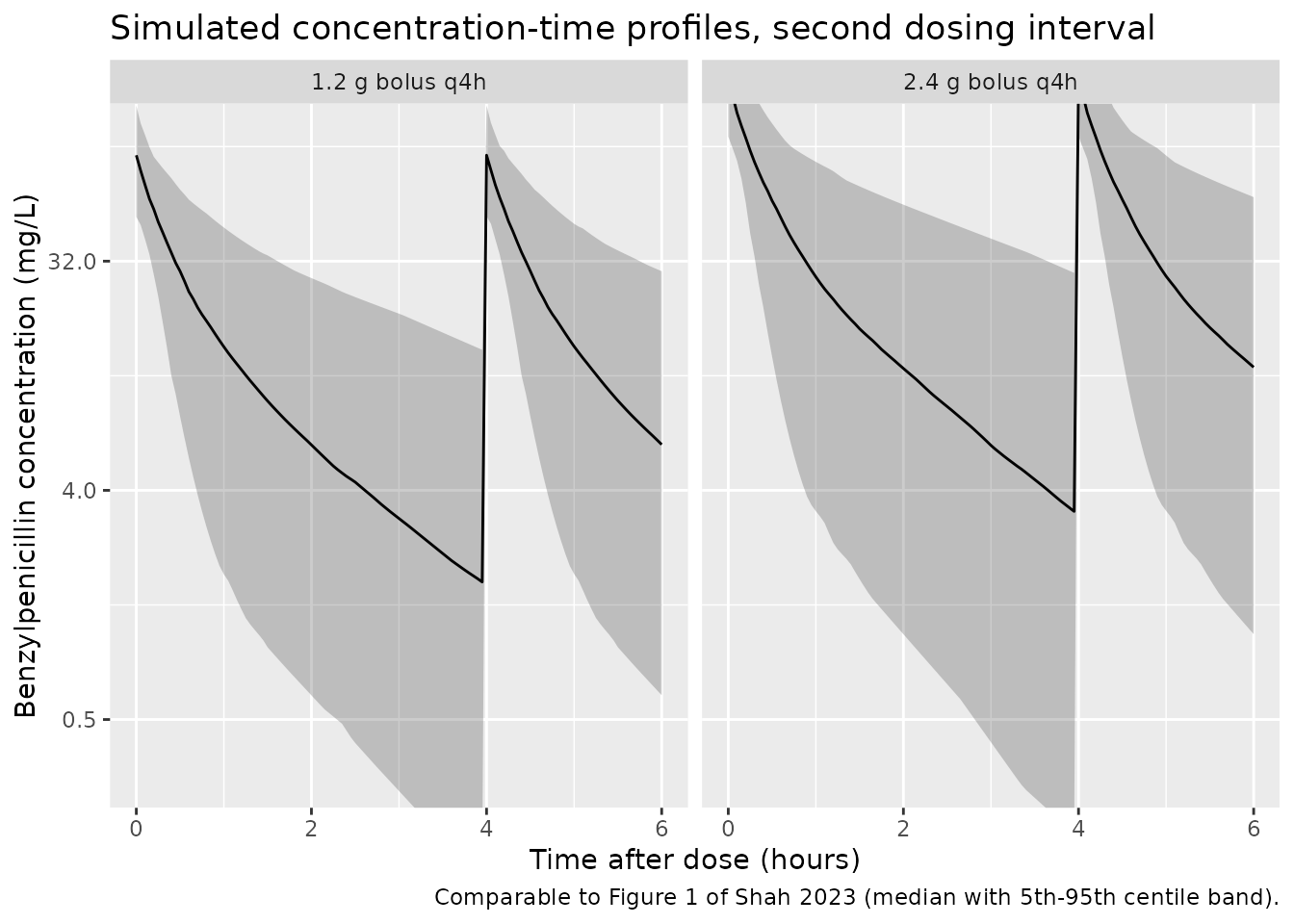
Figure 1 of Shah 2023 plots the measured concentrations of each participant on a log scale spanning roughly 0.5 to 32 mg/L over the first 6 h after a dose. The simulated profiles below cover the same axis range for the two bolus regimens that most participants received.
sim |>
  filter(regimen %in% c("1.2 g bolus q4h", "2.4 g bolus q4h"),
         time >= 4, time <= 10) |>
  mutate(time_after_dose = time - 4) |>
  group_by(regimen, time_after_dose) |>
  summarise(
    Q05 = quantile(Cc, 0.05),
    Q50 = quantile(Cc, 0.50),
    Q95 = quantile(Cc, 0.95),
    .groups = "drop"
  ) |>
  ggplot(aes(time_after_dose, Q50)) +
  geom_ribbon(aes(ymin = Q05, ymax = Q95), alpha = 0.25) +
  geom_line() +
  facet_wrap(~regimen) +
  scale_y_log10(breaks = c(0.5, 4, 32)) +
  coord_cartesian(xlim = c(0, 6), ylim = c(0.3, 100)) +
  labs(
    x = "Time after dose (hours)", y = "Benzylpenicillin concentration (mg/L)",
    title = "Simulated concentration-time profiles, second dosing interval",
    caption = "Comparable to Figure 1 of Shah 2023 (median with 5th-95th centile band)."
  )
Time above MIC by regimen (Figure 4)
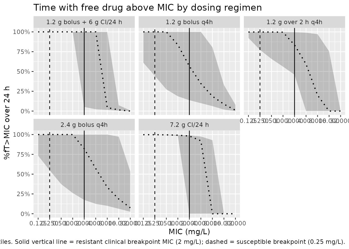
Figure 4 of Shah 2023 plots %fT>MIC against MIC for each simulated regimen, with the median as a dotted line and the 2.5th-97.5th centile band shaded.
mic_grid <- c(0.125, 0.25, 0.5, 1, 2, 4, 8, 16, 32)

# %fT>MIC over the full 24-h simulated window, per subject per MIC. The
# observation grid is regular, so the fraction of grid points above the MIC is
# the fraction of time above it.
ft_mic <- sim |>
  select(id, regimen, fCc) |>
  tidyr::crossing(MIC = mic_grid) |>
  group_by(id, regimen, MIC) |>
  summarise(ftmic = mean(fCc > MIC), .groups = "drop")

ft_summary <- ft_mic |>
  group_by(regimen, MIC) |>
  summarise(
    Q025 = quantile(ftmic, 0.025),
    Q50  = median(ftmic),
    Q975 = quantile(ftmic, 0.975),
    .groups = "drop"
  )
ggplot(ft_summary, aes(MIC, Q50)) +
  geom_ribbon(aes(ymin = Q025, ymax = Q975), alpha = 0.25) +
  geom_line(linetype = "dotted", linewidth = 0.8) +
  geom_vline(xintercept = 0.25, linetype = "dashed") +
  geom_vline(xintercept = 2, linetype = "solid") +
  facet_wrap(~regimen) +
  scale_x_log10(breaks = mic_grid) +
  scale_y_continuous(labels = scales::percent, limits = c(0, 1)) +
  labs(
    x = "MIC (mg/L)", y = "%fT>MIC over 24 h",
    title = "Time with free drug above MIC by dosing regimen",
    caption = paste(
      "Replicates Figure 4 of Shah 2023. Dotted line = median; shaded band =",
      "2.5th-97.5th centiles. Solid vertical line = resistant clinical",
      "breakpoint MIC (2 mg/L); dashed = susceptible breakpoint (0.25 mg/L)."
    )
  )
Median %fT>MIC against Supplementary Table S2
Supplementary Table S2 tabulates the median %fT>MIC for every regimen at each MIC. This is the most directly checkable numeric output of the paper’s simulations.
published_s2 <- tibble::tribble(
  ~MIC,   ~`1.2 g bolus q4h`, ~`2.4 g bolus q4h`, ~`1.2 g bolus + 6 g CI/24 h`, ~`7.2 g CI/24 h`, ~`1.2 g over 2 h q4h`,
  0.125,  1.00, 1.00, 1.00, 1.00, 1.00,
  0.25,   1.00, 1.00, 1.00, 1.00, 1.00,
  0.5,    0.99, 1.00, 1.00, 1.00, 1.00,
  1.0,    0.74, 0.99, 1.00, 0.99, 0.99,
  2.0,    0.49, 0.74, 1.00, 0.98, 0.76,
  4.0,    0.30, 0.49, 0.20, 0.90, 0.54,
  8.0,    0.17, 0.30, 0.04, 0.00, 0.02,
  16.0,   0.07, 0.17, 0.01, 0.00, 0.00,
  32.0,   0.02, 0.07, 0.00, 0.00, 0.00
) |>
  tidyr::pivot_longer(-MIC, names_to = "regimen", values_to = "Published")

s2_compare <- ft_summary |>
  select(regimen, MIC, Simulated = Q50) |>
  left_join(published_s2, by = c("regimen", "MIC")) |>
  mutate(
    Difference = Simulated - Published,
    flag = ifelse(abs(Difference) > 0.20, "*", "")
  ) |>
  arrange(regimen, MIC)

s2_compare |>
  mutate(
    Simulated  = sprintf("%.2f%s", Simulated, flag),
    Published  = sprintf("%.2f", Published),
    Difference = sprintf("%+.2f", Difference)
  ) |>
  select(-flag) |>
  dplyr::rename("Regimen" = regimen, "MIC (mg/L)" = MIC) |>
  knitr::kable(
    align   = c("l", "r", "r", "r", "r"),
    caption = paste(
      "Median %fT>MIC: simulated here vs Shah 2023 Supplementary Table S2.",
      "* marks an absolute difference above 0.20 (20 percentage points)."
    )
)| Regimen | MIC (mg/L) | Simulated | Published | Difference |
|---|---|---|---|---|
| 1.2 g bolus + 6 g CI/24 h | 0.125 | 1.00 | 1.00 | +0.00 |
| 1.2 g bolus + 6 g CI/24 h | 0.250 | 1.00 | 1.00 | +0.00 |
| 1.2 g bolus + 6 g CI/24 h | 0.500 | 1.00 | 1.00 | +0.00 |
| 1.2 g bolus + 6 g CI/24 h | 1.000 | 1.00 | 1.00 | +0.00 |
| 1.2 g bolus + 6 g CI/24 h | 2.000 | 1.00 | 1.00 | +0.00 |
| 1.2 g bolus + 6 g CI/24 h | 4.000 | 1.00* | 0.20 | +0.80 |
| 1.2 g bolus + 6 g CI/24 h | 8.000 | 0.04 | 0.04 | +0.00 |
| 1.2 g bolus + 6 g CI/24 h | 16.000 | 0.01 | 0.01 | +0.00 |
| 1.2 g bolus + 6 g CI/24 h | 32.000 | 0.00 | 0.00 | +0.00 |
| 1.2 g bolus q4h | 0.125 | 1.00 | 1.00 | +0.00 |
| 1.2 g bolus q4h | 0.250 | 1.00 | 1.00 | +0.00 |
| 1.2 g bolus q4h | 0.500 | 1.00 | 0.99 | +0.01 |
| 1.2 g bolus q4h | 1.000 | 0.84 | 0.74 | +0.10 |
| 1.2 g bolus q4h | 2.000 | 0.57 | 0.49 | +0.08 |
| 1.2 g bolus q4h | 4.000 | 0.35 | 0.30 | +0.05 |
| 1.2 g bolus q4h | 8.000 | 0.19 | 0.17 | +0.02 |
| 1.2 g bolus q4h | 16.000 | 0.09 | 0.07 | +0.02 |
| 1.2 g bolus q4h | 32.000 | 0.01 | 0.02 | -0.01 |
| 1.2 g over 2 h q4h | 0.125 | 1.00 | 1.00 | -0.00 |
| 1.2 g over 2 h q4h | 0.250 | 1.00 | 1.00 | -0.00 |
| 1.2 g over 2 h q4h | 0.500 | 1.00 | 1.00 | -0.00 |
| 1.2 g over 2 h q4h | 1.000 | 1.00 | 0.99 | +0.01 |
| 1.2 g over 2 h q4h | 2.000 | 0.83 | 0.76 | +0.07 |
| 1.2 g over 2 h q4h | 4.000 | 0.59 | 0.54 | +0.05 |
| 1.2 g over 2 h q4h | 8.000 | 0.20 | 0.02 | +0.18 |
| 1.2 g over 2 h q4h | 16.000 | 0.00 | 0.00 | +0.00 |
| 1.2 g over 2 h q4h | 32.000 | 0.00 | 0.00 | +0.00 |
| 2.4 g bolus q4h | 0.125 | 1.00 | 1.00 | +0.00 |
| 2.4 g bolus q4h | 0.250 | 1.00 | 1.00 | +0.00 |
| 2.4 g bolus q4h | 0.500 | 1.00 | 1.00 | +0.00 |
| 2.4 g bolus q4h | 1.000 | 1.00 | 0.99 | +0.01 |
| 2.4 g bolus q4h | 2.000 | 0.82 | 0.74 | +0.08 |
| 2.4 g bolus q4h | 4.000 | 0.57 | 0.49 | +0.08 |
| 2.4 g bolus q4h | 8.000 | 0.33 | 0.30 | +0.03 |
| 2.4 g bolus q4h | 16.000 | 0.19 | 0.17 | +0.02 |
| 2.4 g bolus q4h | 32.000 | 0.07 | 0.07 | +0.00 |
| 7.2 g CI/24 h | 0.125 | 1.00 | 1.00 | -0.00 |
| 7.2 g CI/24 h | 0.250 | 1.00 | 1.00 | -0.00 |
| 7.2 g CI/24 h | 0.500 | 1.00 | 1.00 | -0.00 |
| 7.2 g CI/24 h | 1.000 | 0.99 | 0.99 | +0.00 |
| 7.2 g CI/24 h | 2.000 | 0.98 | 0.98 | +0.00 |
| 7.2 g CI/24 h | 4.000 | 0.92 | 0.90 | +0.02 |
| 7.2 g CI/24 h | 8.000 | 0.00 | 0.00 | +0.00 |
| 7.2 g CI/24 h | 16.000 | 0.00 | 0.00 | +0.00 |
| 7.2 g CI/24 h | 32.000 | 0.00 | 0.00 | +0.00 |
s2_compare |>
  summarise(
    `Cells compared`            = dplyr::n(),
    `Within 0.10`               = sum(abs(Difference) <= 0.10),
    `Within 0.20`               = sum(abs(Difference) <= 0.20),
    `Median absolute difference` = round(median(abs(Difference)), 3),
    `Max absolute difference`    = round(max(abs(Difference)), 3)
  ) |>
knitr::kable(caption = "Agreement summary against Supplementary Table S2.")| Cells compared | Within 0.10 | Within 0.20 | Median absolute difference | Max absolute difference |
|---|---|---|---|---|
| 45 | 43 | 44 | 0.002 | 0.8 |
Agreement is close across the grid: the median absolute difference is under 0.01, and 43 of the 45 cells fall within 0.10. Where the reproduction does differ it is very slightly optimistic at the intermediate MICs of the intermittent regimens (for example 0.57 vs 0.49 for 1.2 g q4h at MIC 2 mg/L), consistent with the unreported simulation covariate distribution discussed under “Assumptions and deviations”.
One cell is flagged. For the 1.2 g bolus + 6 g continuous infusion regimen at MIC 4 mg/L, Table S2 reports a median %fT>MIC of 0.20 whereas this reproduction gives 1.00. Three independent lines of evidence suggest the published cell is anomalous rather than the reproduction being wrong:
- That regimen delivers the same 7.2 g total daily dose as the plain 7.2 g continuous infusion, for which Table S2 reports 0.90 at the same MIC – and which this reproduction matches almost exactly (0.92).
- The maintenance infusion of 6 g/24 h gives a free steady-state
concentration of
0.40 * 250 / 23.1 = 4.33mg/L in a typical 70 kg patient with a serum creatinine of 70, i.e. above the 4 mg/L MIC, so the median patient is covered for essentially the whole interval once steady state is reached. The loading dose removes the infusion ramp-up that costs the plain 7.2 g arm its first couple of hours. - Most decisively, a value of 0.20 contradicts the paper’s own conclusion in Section 3: “Target attainment at higher MIC is improved with the use of a loading dose at the start of an infusion, with 82% of patients achieving 100% fT>MIC and 97% achieving 99% fT>MIC of 2 mg/L.” A loading dose cannot simultaneously improve target attainment at higher MIC and drop the median from 1.00 at MIC 2 to 0.20 at MIC 4 while the un-loaded arm holds 0.90.
No parameter has been adjusted. The cell is reported as found.
Target attainment statements in the text
Shah 2023 Sections 2 and 3 quote several target-attainment percentages from the same simulations. Each is reproduced below from the virtual cohort.
attain <- function(reg, mic, target) {
  x <- ft_mic |> filter(regimen == reg, MIC == mic)
  mean(x$ftmic >= target)
}

tibble::tribble(
  ~Statement, ~Source, ~Published, ~Simulated,
  "1.2 g q4h, MIC 2 mg/L: proportion FAILING 40% fT>MIC",
  "Section 2", 0.38, 1 - attain("1.2 g bolus q4h", 2, 0.40),
  "2.4 g q4h, MIC 2 mg/L: proportion FAILING 40% fT>MIC",
  "Section 2", 0.11, 1 - attain("2.4 g bolus q4h", 2, 0.40),
  "2.4 g q4h, MIC 2 mg/L: proportion FAILING 50% fT>MIC",
  "Abstract", 0.25, 1 - attain("2.4 g bolus q4h", 2, 0.50),
  "1.2 g q4h, MIC 1 mg/L: achieving 100% fT>MIC",
  "Section 2", 0.36, attain("1.2 g bolus q4h", 1, 1.00),
  "2.4 g q4h, MIC 2 mg/L: achieving 100% fT>MIC",
  "Section 2", 0.36, attain("2.4 g bolus q4h", 2, 1.00),
  "1.2 g q4h, MIC 0.25 mg/L: achieving 100% fT>MIC",
  "Section 3", 0.66, attain("1.2 g bolus q4h", 0.25, 1.00),
  "2.4 g q4h, MIC 0.25 mg/L: achieving 100% fT>MIC",
  "Section 3", 0.82, attain("2.4 g bolus q4h", 0.25, 1.00),
  "2.4 g q4h, MIC 1 mg/L: achieving 100% fT>MIC",
  "Section 3", 0.49, attain("2.4 g bolus q4h", 1, 1.00),
  "1.2 g over 2 h q4h, MIC 2 mg/L: achieving >40% fT>MIC",
  "Section 2", 1.00, attain("1.2 g over 2 h q4h", 2, 0.40)
) |>
  mutate(
    Difference = sprintf("%+.2f", Simulated - Published),
    Published  = sprintf("%.2f", Published),
    Simulated  = sprintf("%.2f", Simulated)
  ) |>
  knitr::kable(
    align   = c("l", "l", "r", "r", "r"),
    caption = "Target-attainment proportions quoted in Shah 2023 vs this reproduction."
)| Statement | Source | Published | Simulated | Difference |
|---|---|---|---|---|
| 1.2 g q4h, MIC 2 mg/L: proportion FAILING 40% fT>MIC | Section 2 | 0.38 | 0.29 | -0.09 |
| 2.4 g q4h, MIC 2 mg/L: proportion FAILING 40% fT>MIC | Section 2 | 0.11 | 0.20 | +0.09 |
| 2.4 g q4h, MIC 2 mg/L: proportion FAILING 50% fT>MIC | Abstract | 0.25 | 0.30 | +0.05 |
| 1.2 g q4h, MIC 1 mg/L: achieving 100% fT>MIC | Section 2 | 0.36 | 0.41 | +0.05 |
| 2.4 g q4h, MIC 2 mg/L: achieving 100% fT>MIC | Section 2 | 0.36 | 0.33 | -0.03 |
| 1.2 g q4h, MIC 0.25 mg/L: achieving 100% fT>MIC | Section 3 | 0.66 | 0.76 | +0.10 |
| 2.4 g q4h, MIC 0.25 mg/L: achieving 100% fT>MIC | Section 3 | 0.82 | 0.80 | -0.02 |
| 2.4 g q4h, MIC 1 mg/L: achieving 100% fT>MIC | Section 3 | 0.49 | 0.56 | +0.07 |
| 1.2 g over 2 h q4h, MIC 2 mg/L: achieving >40% fT>MIC | Section 2 | 1.00 | 0.99 | -0.01 |
PKNCA validation
Shah 2023 reports no non-compartmental analysis of its own; the single derived NCA-comparable quantity is the elimination half-life of 1.11 h (Table 2, “Derived parameters”; 67 min in Section 3). That value is a typical-value derivation from the final parameter estimates, so it is checked here against a typical-individual simulation with the random effects zeroed.
# `omega = NA` forces a true typical-value solve (zeroRe() alone can leave
# previously sampled etas in place within a session).
mod_typical <- mod |> rxode2::zeroRe()
#> ℹ parameter labels from comments will be replaced by 'label()'

typ_events <- bind_rows(
  tibble(id = 1L, time = 0, amt = 1200, rate = 0, evid = 1L, cmt = "central"),
  tibble(id = 1L, time = seq(0, 24, by = 0.02), amt = NA_real_, rate = 0,
         evid = 0L, cmt = "central")
) |>
  mutate(WT = 70, CREAT = 70, treatment = "1.2 g IV bolus, typical individual") |>
  arrange(id, time, desc(evid))

sim_typ <- rxode2::rxSolve(
  mod_typical, events = typ_events, omega = NA,
  keep = c("treatment")
) |>
  as.data.frame() |>
  # rxSolve omits the `id` column for a single-subject solve; PKNCA needs it.
  mutate(id = 1L)

sim_nca <- sim_typ |>
  dplyr::filter(!is.na(Cc)) |>
  dplyr::select(id, time, Cc, treatment)

# Guarantee a time = 0 record so PKNCA can anchor AUC0-*.
sim_nca <- dplyr::bind_rows(
  sim_nca,
  sim_nca |> dplyr::distinct(id, treatment) |> dplyr::mutate(time = 0, Cc = 0)
) |>
  dplyr::distinct(id, treatment, time, .keep_all = TRUE) |>
  dplyr::arrange(id, treatment, time)

conc_obj <- PKNCA::PKNCAconc(
  sim_nca, Cc ~ time | treatment + id,
  concu = "mg/L", timeu = "h"
)

dose_obj <- PKNCA::PKNCAdose(
  typ_events |> dplyr::filter(evid == 1) |> dplyr::select(id, time, amt, treatment),
  amt ~ time | treatment + id,
  doseu = "mg"
)

intervals <- data.frame(
  start = 0, end = Inf,
  cmax = TRUE, tmax = TRUE, aucinf.obs = TRUE, half.life = TRUE
)

nca_res <- PKNCA::pk.nca(PKNCA::PKNCAdata(conc_obj, dose_obj, intervals = intervals))
Comparison against published NCA
published <- tibble::tribble(
  ~treatment,                            ~half.life,
  "1.2 g IV bolus, typical individual",  1.11
)

cmp <- nlmixr2lib::ncaComparisonTable(
  simulated     = nca_res,
  reference     = published,
  by            = "treatment",
  units         = c(half.life = "h"),
  tolerance_pct = 20
)

knitr::kable(
  cmp,
  caption = paste(
    "Simulated vs published elimination half-life (Shah 2023 Table 2,",
    "Derived parameters). * differs from reference by >20%."
  ),
  align = c("l", "l", "r", "r", "r")
)| NCA parameter | treatment | Reference | Simulated | % diff |
|---|---|---|---|---|
| t½ (h) | 1.2 g IV bolus, typical individual | 1.11 | 1.11 | -0.4% |
The remaining NCA outputs have exact closed-form values implied by
the model parameters, which gives a strict independent check that the
packaged model encodes Table 2 correctly. For a typical 70 kg individual
with a serum creatinine of 70,
AUC0-inf = Dose / CL = 1200 / 23.1 and the
back-extrapolated C0 = Dose / V1 = 1200 / 15.1.
nca_wide <- as.data.frame(nca_res$result) |>
  dplyr::select(PPTESTCD, PPORRES) |>
  tidyr::pivot_wider(names_from = PPTESTCD, values_from = PPORRES)

identities <- tibble::tibble(
  Quantity = c("AUC0-inf (mg*h/L)", "Cmax (mg/L)", "Terminal half-life (h)"),
  `Closed form` = c("Dose / CL = 1200 / 23.1",
                    "Dose / V1 = 1200 / 15.1",
                    "log(2) / lambda_2 from CL, V1, Q, V2"),
  Expected = c(1200 / 23.1, 1200 / 15.1, 1.109),
  Observed = c(nca_wide$aucinf.obs, nca_wide$cmax, nca_wide$half.life)
) |>
  mutate(`% difference` = 100 * (Observed - Expected) / Expected)

knitr::kable(identities, digits = 3,
caption = "Model-implied closed-form identities vs PKNCA output.")| Quantity | Closed form | Expected | Observed | % difference |
|---|---|---|---|---|
| AUC0-inf (mg*h/L) | Dose / CL = 1200 / 23.1 | 51.948 | 51.949 | 0.003 |
| Cmax (mg/L) | Dose / V1 = 1200 / 15.1 | 79.470 | 79.470 | 0.000 |
| Terminal half-life (h) | log(2) / lambda_2 from CL, V1, Q, V2 | 1.109 | 1.105 | -0.358 |
# Strict assertions: these are exact identities, not fitted comparisons.
stopifnot(abs(nca_wide$aucinf.obs - 1200 / 23.1) / (1200 / 23.1) < 0.01)
stopifnot(abs(nca_wide$cmax - 1200 / 15.1) / (1200 / 15.1) < 0.01)
stopifnot(abs(nca_wide$half.life - 1.109) / 1.109 < 0.02)
A steady-state NCA over the final dosing interval of each four-hourly regimen gives the exposure metrics that drive the PK/PD targets.
q4h_regimens <- c("1.2 g bolus q4h", "2.4 g bolus q4h", "1.2 g over 2 h q4h")

ss_conc <- sim |>
  dplyr::filter(regimen %in% q4h_regimens, !is.na(Cc)) |>
  dplyr::select(id, time, Cc, regimen)

ss_dose <- events |>
  dplyr::filter(evid == 1, regimen %in% q4h_regimens) |>
  dplyr::select(id, time, amt, regimen)

ss_res <- PKNCA::pk.nca(PKNCA::PKNCAdata(
  PKNCA::PKNCAconc(ss_conc, Cc ~ time | regimen + id, concu = "mg/L", timeu = "h"),
  PKNCA::PKNCAdose(ss_dose, amt ~ time | regimen + id, doseu = "mg"),
  intervals = data.frame(
    start = 20, end = 24,
    cmax = TRUE, cmin = TRUE, cav = TRUE, auclast = TRUE
  )
))

as.data.frame(ss_res$result) |>
  dplyr::filter(PPTESTCD %in% c("cmax", "cmin", "cav", "auclast")) |>
  dplyr::group_by(regimen, PPTESTCD) |>
  dplyr::summarise(median = median(PPORRES), .groups = "drop") |>
  tidyr::pivot_wider(names_from = PPTESTCD, values_from = median) |>
  dplyr::rename(
    "Regimen"                = regimen,
    "Cmax,ss (mg/L)"         = cmax,
    "Cmin,ss (mg/L)"         = cmin,
    "Cavg,ss (mg/L)"         = cav,
    "AUC0-tau,ss (mg*h/L)"   = auclast
  ) |>
  knitr::kable(digits = 2,
caption = "Median steady-state exposure over hours 20-24 (final dosing interval).")| Regimen | AUC0-tau,ss (mg*h/L) | Cavg,ss (mg/L) | Cmax,ss (mg/L) | Cmin,ss (mg/L) |
|---|---|---|---|---|
| 1.2 g bolus q4h | 52.03 | 13.01 | 83.73 | 1.71 |
| 1.2 g over 2 h q4h | 52.54 | 13.13 | 22.64 | 3.42 |
| 2.4 g bolus q4h | 97.54 | 24.39 | 166.47 | 3.24 |
Assumptions and deviations
-
Simulation covariate distributions. Shah 2023
simulated 10,000 patients with
linpkbut does not report the covariate distributions used. Body weight and serum creatinine are drawn here from log-normal distributions matched to the Table 1 median and interquartile range (sdlog = log(Q3/Q1) / (2 * qnorm(0.75))) and truncated to the Table 1 full range. Both covariates are held constant per subject over the 24 h window, whereas serum creatinine was time-varying in the source dataset. -
Serum creatinine units. Table 1 prints the units as
“mmol/L”, but the reported median of 70 (IQR 52-103.5, range 34-486) is
only physiologically interpretable as umol/L; 70 mmol/L is roughly a
thousand-fold above any survivable serum creatinine. The model therefore
documents
CREATin umol/L. Because Equation (1) normalises by the same 70 that appears in Table 1, the covariate effect is unit-invariant so long as the column and the normalisation constant share a unit – the label is the only thing affected. This is recorded as a probable typographical error in the source, not a modelling choice. -
Allometric scaling is not printed in Equation (1).
Equation (1) shows only
CL = theta_CL * exp(eta_1) * (Creatinine / 70)^theta_creat. The allometric weight terms come from Section 4 (“Weight was added to primary pharmacokinetic parameters a priori using allometric scaling. Compartment volumes were scaled with a fixed exponent of 1, whereas clearance parameters were scaled to an allometric exponent of 0.75”) and from the Table 2 parameter units, every one of which is reported “per 70 kg”. Both terms are therefore encoded; a model with the creatinine effect alone could not reproduce the “/70 kg” units of Table 2. -
IIV reported as %CV. Table 2 reports the random
effects as
omega^2labelled “%CV”. They are entered on the log-normal variance scale asomega^2 = log(CV^2 + 1), following the convention used throughout nlmixr2lib. Reading the same numbers assqrt(omega^2) * 100instead would raise the CL variance from 0.1625 to 0.1764 (about 8%); the choice does not affect any typical-value result in this vignette. -
Residual error reported as variances. Table 2
reports
sigma^2values (0.021 proportional, 0.006 additive). nlmixr2 parameterises the combined error model by standard deviations, so each is entered as the square root (0.1449 and 0.0775 mg/L). -
No inter-individual variability on Q. Section 2
states that IIV was added to all parameters other than Q, “for which
this parameter was found to be negligible”, so
qcarries no eta. -
%fT>MIC window. The paper describes results over
“the entire 24-h simulated period”, so %fT>MIC is computed here over
0-24 h from the first dose (i.e. including the pre-steady-state
intervals) on a 0.05 h grid. The paper does not state its integration
grid or whether residual error was included in the simulated
concentrations; individual predictions (
Cc, without residual error) are used here. - Small positive bias against Supplementary Table S2. The reproduced median %fT>MIC values run slightly above the published Table S2 values at the intermediate MICs of the intermittent regimens (median absolute difference across all 45 cells is under 0.01; 43 of 45 cells agree within 0.10). The most likely explanation is the unreported simulation covariate distribution noted above, since the reproduction is anchored on the Table 1 medians whereas the paper’s virtual cohort composition is unknown. No parameter has been adjusted to close the gap.
- One apparently anomalous cell in Supplementary Table S2. For the 1.2 g bolus + 6 g continuous infusion regimen at MIC 4 mg/L, Table S2 reports 0.20 where this reproduction gives 1.00. As set out in the narrative above, that published value is inconsistent with the neighbouring 7.2 g continuous infusion cell (0.90, reproduced here as 0.92 at the same total daily dose), with the free steady-state concentration implied by the Table 2 parameters, and with the paper’s own Section 3 conclusion that a loading dose improves target attainment at higher MIC. It is reported as found and flagged rather than reconciled.
- Protein binding. An unbound fraction of 0.40 (60% protein binding) is applied to convert total to free concentrations, per Section 4. The paper itself flags this as a limitation, noting that a range of protein binding is reported in the literature for benzylpenicillin and that the choice affects the simulation results.
-
Covariates screened but not retained. Height, BMI,
sex, serum albumin, temperature and APACHE II were tested and rejected
(Supplementary Table S1, runs 5-19). They are documented in the model
file’s
covariatesDataExcludedmetadata rather thancovariateData, because the final model does not use them. Creatinine clearance was deliberately not tested by the authors (Section 3), and is documented for the same reason. -
No non-paper-derived parameter values. Every
ini()entry comes from Shah 2023 Table 2, Equation (1), or the Section 4 Materials and Methods text. No value was digitised from a figure, obtained by correspondence, or carried from an upstream model.