Simurosertib (Zhou 2022) • nlmixr2lib

Model and source

Citation: Zhou X, Ouerdani A, Diderichsen PM, Gupta N. Population Pharmacokinetics of TAK-931, a Cell Division Cycle 7 Kinase Inhibitor, in Patients With Advanced Solid Tumors. J Clin Pharmacol. 2022;62(3):422-433. doi:10.1002/jcph.1974. PMC9297904. Open Access under CC BY-NC 4.0. Parameter estimates are in Table 3 and Equation 7; the model schema is Supplemental Figure S1 and the simulated day-1 / day-14 exposure summaries used for validation are Supplemental Table S2.
Description: Two-compartment population pharmacokinetic model for oral simurosertib (TAK-931, a cell division cycle 7 kinase inhibitor) in 198 adults with advanced solid tumors, from Zhou 2022. Absorption is a chain of two transit compartments in which the absorption rate constant equals the transit rate constant (ktr = 2 / MTT); elimination is first-order linear. Creatinine clearance (Cockcroft-Gault) and body weight enter apparent clearance as power functions centred on 90.45 mL/min and 65.95 kg, and body weight also scales the apparent central volume and intercompartmental clearance. Between-subject variability is carried on apparent clearance and the mean transit time; residual error is additive on log-transformed concentrations.
Article: https://doi.org/10.1002/jcph.1974 (open access, PMC9297904)

Simurosertib is the INN of TAK-931, the name used throughout the paper.

Population

The model was fit to 2678 post-dose plasma concentrations from 198 adults with advanced nonhematologic solid tumors pooled from three Takeda studies (Zhou 2022 Table 1): the first-in-human phase 1 dose escalation TAK-931-1002 in Japan (n = 80; 20-150 mg once daily on four on/off schedules), the phase 1 capsule-versus-tablet relative-bioavailability crossover TAK-931-1003 (n = 20; 80 mg), and the phase 2 study TAK-931-2001 (n = 98; 50 mg once daily, 14 days on / 7 days off). Table 2 gives the baseline demographics: median age 61 years (36-88), median body weight 65.8 kg (29.8-127), median Cockcroft-Gault creatinine clearance 89.9 mL/min (35-204), 60% female, and 55.1% Asian, 33.3% White, 4% Black or African American and 7.6% other race. Half the cohort (50.5%) had normal renal function, 32.8% mild and 17.7% moderate renal impairment; 19.7% had mild hepatic impairment.

The same information is available programmatically:

str(rxode2::rxode(readModelDb("Zhou_2022_simurosertib"))$population)
#> ℹ parameter labels from comments will be replaced by 'label()'
#> List of 16
#>  $ species       : chr "human"
#>  $ n_subjects    : int 198
#>  $ n_studies     : int 3
#>  $ n_observations: int 2678
#>  $ age_range     : chr "36-88 years"
#>  $ age_median    : chr "61 years"
#>  $ weight_range  : chr "29.8-127 kg"
#>  $ weight_median : chr "65.8 kg"
#>  $ crcl_range    : chr "35-204 mL/min (Cockcroft-Gault)"
#>  $ crcl_median   : chr "89.9 mL/min"
#>  $ sex_female_pct: num 60
#>  $ race_ethnicity: Named num [1:4] 55.1 33.3 4 7.6
#>   ..- attr(*, "names")= chr [1:4] "Asian" "White" "Black or African American" "Other"
#>  $ disease_state : chr "Adults with advanced nonhematologic solid tumors, including metastatic pancreatic and colorectal cancer. Renal "| __truncated__
#>  $ dose_range    : chr "Oral simurosertib 20-150 mg once daily on several on/off schedules (14 days on / 7 off, 7 on / 7 off, 21 days c"| __truncated__
#>  $ regions       : chr "Japan (first-in-human phase 1 TAK-931-1002) and Western sites (phase 2 TAK-931-2001)."
#>  $ notes         : chr "Pooled from studies TAK-931-1002 (phase 1, n = 80; NCT02699749), TAK-931-1003 (phase 1 relative bioavailability"| __truncated__

Source trace

Equation / parameter	Value	Source location
`lcl` (CL/F)	log(38.0) L/h	Table 3; Equation 7
`lvc` (Vc/F)	log(194) L	Table 3; Equation 7
`lq` (Q/F)	log(7.71) L/h	Table 3; Equation 7
`lvp` (Vp/F)	log(140) L	Table 3
`lmtt` (MTT)	log(0.756) h	Table 3
`e_crcl_cl`	0.325	Table 3; Equation 7
`e_wt_cl`	0.484	Table 3; Equation 7
`e_wt_vc`	0.867	Table 3; Equation 7
`e_wt_q`	0.938	Table 3; Equation 7
`etalcl`	0.050245 = log(0.227^2 + 1)	Table 3 (22.7% CV) and its footnote CV = sqrt(exp(omega^2) - 1)
`etalmtt`	0.357909 = log(0.656^2 + 1)	Table 3 (65.6% CV)
`expSd`	0.499	Table 3 ‘Additive residual error (standard deviation) in log scale’; Methods Equation 2
Covariate references 90.45 mL/min, 65.95 kg	n/a	Equation 7; Methods ‘Model-Based Simulations’; Figure 5 legend
Power covariate form	n/a	Methods Equation 4
Log-normal IIV	n/a	Methods Equation 1
`depot -> transit1 -> transit2 -> central`, ka = ktr	n/a	Supplemental Figure S1; Results ‘Base Model Development’
`ktr = 2 / mtt`	n/a	Not printed; chosen against Supplemental Table S2 (see below)
Two-compartment disposition, linear elimination	n/a	Results ‘Base Model Development’; Supplemental Figure S1

Virtual cohort

The individual data are not public. The virtual cohort draws body weight and creatinine clearance from log-normal distributions centred on the Table 2 medians and truncated to the Table 2 ranges. The two covariates are drawn independently because the paper does not report their correlation.

# set.seed() seeds R's RNG (the covariates); rxSetSeed() seeds rxode2's
# random effects. rxode2's streams are partitioned per solver thread, so the
# cohort differs between machines with different thread counts -- every
# assertion below is written to hold for any cohort.
set.seed(20220303)
rxode2::rxSetSeed(20220303)

n_sub <- 200
rtrunc_lnorm <- function(n, median, sdlog, lower, upper) {
  out <- numeric(0)
  while (length(out) < n) {
    x <- exp(rnorm(2 * n, log(median), sdlog))
    out <- c(out, x[x >= lower & x <= upper])
  }
  out[seq_len(n)]
}
cohort <- tibble(
  id = seq_len(n_sub),
  WT = rtrunc_lnorm(n_sub, 65.8, 0.22, 29.8, 127),
  CRCL = rtrunc_lnorm(n_sub, 89.9, 0.33, 35, 204)
)

summary(cohort[, c("WT", "CRCL")])
#>        WT              CRCL       
#>  Min.   : 35.42   Min.   : 36.23  
#>  1st Qu.: 55.04   1st Qu.: 70.32  
#>  Median : 63.78   Median : 89.09  
#>  Mean   : 65.81   Mean   : 93.19  
#>  3rd Qu.: 74.40   3rd Qu.:111.66  
#>  Max.   :113.59   Max.   :201.42

Simulation

The regimen is 50 mg once daily for 14 days, the phase 2 dose used for Figure 4 and Supplemental Table S2. Day 1 and day 14 are sampled every 0.1 h for NCA; the days in between are sampled every 0.5 h for Figure 4.

dose_times <- 24 * (0:13)
obs_times <- sort(unique(c(
  seq(0, 24, by = 0.1),
  seq(24, 312, by = 0.5),
  seq(312, 336, by = 0.1)
)))

# Dose rows go into the depot; observation rows sit on the central ODE state
# (Cc is returned at every observation row).
doses <- cohort |>
  tidyr::crossing(time = dose_times) |>
  dplyr::mutate(evid = 1L, amt = 50, cmt = "depot")
obs <- cohort |>
  tidyr::crossing(time = obs_times) |>
  dplyr::mutate(evid = 0L, amt = NA_real_, cmt = "central")
events <- dplyr::bind_rows(doses, obs) |>
  dplyr::arrange(id, time, dplyr::desc(evid))
stopifnot(!anyDuplicated(events[, c("id", "time", "evid")]))

mod <- readModelDb("Zhou_2022_simurosertib")
sim <- rxode2::rxSolve(mod, events = events, keep = c("WT", "CRCL")) |>
  as.data.frame()
#> ℹ parameter labels from comments will be replaced by 'label()'
# Cc is the individual prediction (between-subject variability, no residual
# error), which is what the paper's simulated summaries describe; the
# residual-error draw is in the separate `sim` column.
stopifnot(!anyNA(sim$Cc))

Replicate published figures

Figure 4 – 50 mg once daily for 14 days

# Replicates Figure 4 of Zhou 2022: median and 95% prediction interval of the
# simulated concentrations, 50 mg once daily for 14 days.
sim |>
  dplyr::group_by(time) |>
  dplyr::summarise(
    Q025 = quantile(Cc, 0.025),
    Q50 = median(Cc),
    Q975 = quantile(Cc, 0.975),
    .groups = "drop"
  ) |>
  ggplot(aes(time / 24 + 1, Q50)) +
  geom_ribbon(aes(ymin = Q025, ymax = Q975), fill = "grey60") +
  geom_line() +
  scale_x_continuous(breaks = 1:15) +
  labs(
    x = "Time (days)",
    y = "Simulated simurosertib concentration (ng/mL)",
    title = "Figure 4 -- 50 mg once daily",
    caption = "Replicates Figure 4 of Zhou 2022."
  )

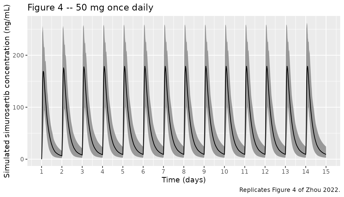
fig4_peaks <- sim |>
  dplyr::filter(time <= 24 | time >= 312) |>
  dplyr::mutate(day = ifelse(time <= 24, "Day 1", "Day 14")) |>
  dplyr::group_by(day, time) |>
  dplyr::summarise(Q50 = median(Cc), Q975 = quantile(Cc, 0.975), .groups = "drop") |>
  dplyr::group_by(day) |>
  dplyr::summarise(
    median_profile_peak = max(Q50),
    p975_profile_peak = max(Q975),
    .groups = "drop"
  )
knitr::kable(fig4_peaks, digits = 1, caption = "Peaks of the simulated median and 97.5th-percentile profiles (ng/mL).")

Peaks of the simulated median and 97.5th-percentile profiles (ng/mL).
day	median_profile_peak	p975_profile_peak
Day 1	169.1	255.9
Day 14	178.8	262.4

The paper’s Figure 4 median profile peaks at about 150 ng/mL on day 1 and 155 ng/mL at steady state, and its 97.5th percentile at about 270 ng/mL (digitised by the maintainers from the plot); steady state is reached within about 3 days. The replicated median-profile peak is about 13% higher than the digitised value (169 vs 150 ng/mL on day 1 in the maintainers’ render). The plotted median is sensitive to the time grid and to how the absorption phase lines up across subjects, so the Cmax distribution in Supplemental Table S2 (next section) is the better-defined comparison.

PKNCA validation

Supplemental Table S2 tabulates the paper’s simulated AUC0-24, average concentration, Cmax and trough concentration on day 1 and day 14 of 50 mg once daily. Each day is put on its own time axis starting at that day’s dose so PKNCA computes the same 0-24 h interval for both.

sim_nca <- sim |>
  dplyr::filter(!is.na(Cc)) |>
  dplyr::filter(time <= 24 | time >= 312) |>
  dplyr::mutate(
    day = ifelse(time <= 24, "Day 1", "Day 14"),
    tday = round(ifelse(day == "Day 1", time, time - 312), 1)
  ) |>
  dplyr::select(id, day, tday, Cc)
# Guarantee a time-zero row per subject and day (the day-1 pre-dose
# concentration is 0; the day-14 pre-dose row is already on the grid).
sim_nca <- dplyr::bind_rows(
  sim_nca,
  sim_nca |> dplyr::distinct(id, day) |> dplyr::mutate(tday = 0, Cc = 0)
) |>
  dplyr::distinct(id, day, tday, .keep_all = TRUE) |>
  dplyr::arrange(id, day, tday)

dose_nca <- sim_nca |>
  dplyr::distinct(id, day) |>
  dplyr::mutate(tday = 0, amt = 50)

conc_obj <- PKNCA::PKNCAconc(sim_nca, Cc ~ tday | day + id)
dose_obj <- PKNCA::PKNCAdose(dose_nca, amt ~ tday | day + id)
intervals <- data.frame(
  start = 0,
  end = 24,
  cmax = TRUE,
  tmax = TRUE,
  auclast = TRUE,
  cav = TRUE,
  clast.obs = TRUE
)
nca_res <- PKNCA::pk.nca(
  PKNCA::PKNCAdata(conc_obj, dose_obj, intervals = intervals)
)
nca_ind <- as.data.frame(nca_res) |>
  dplyr::filter(PPTESTCD %in% c("cmax", "tmax", "auclast", "cav", "clast.obs"))

Comparison against published NCA

The trough is the concentration 24 h after the day’s dose (clast.obs); Table S2 labels it the minimum concentration. Table S2 prints AUC in “ugh/mL”, but its values (1149 and 1280) are ngh/mL: 50 mg divided by a clearance of 38 L/h is 1316 ngh/mL, and Table S2’s own average concentration (47.86 ng/mL) times 24 h is 1149 ngh/mL.

published <- tibble::tribble(
  ~day, ~cmax, ~auclast, ~cav, ~clast.obs,
  "Day 1", 171.1, 1149, 47.86, 6.504,
  "Day 14", 180.8, 1280, 53.32, 9.349
)
cmp <- nlmixr2lib::ncaComparisonTable(
  simulated = nca_ind,
  reference = published,
  by = "day",
  units = c(
    cmax = "ng/mL", auclast = "ng*h/mL", cav = "ng/mL",
    clast.obs = "ng/mL"
  ),
  tolerance_pct = 20
)
knitr::kable(
  cmp,
  caption = paste(
    "Simulated medians vs Zhou 2022 Supplemental Table S2 medians,",
    "50 mg once daily. * differs from reference by >20%."
  )
)

Simulated medians vs Zhou 2022 Supplemental Table S2 medians, 50 mg once daily. * differs from reference by >20%.
NCA parameter	day	Reference	Simulated	% diff
Cmax (ng/mL)	Day 1	171	186	+8.8%
Cmax (ng/mL)	Day 14	181	195	+7.6%
Clast (ng/mL)	Day 1	6.5	6.43	-1.2%
Clast (ng/mL)	Day 14	9.35	9.29	-0.7%
AUClast (ng*h/mL)	Day 1	1150	1210	+5.1%
AUClast (ng*h/mL)	Day 14	1280	1340	+4.9%
Cavg (ng/mL)	Day 1	47.9	50.3	+5.1%
Cavg (ng/mL)	Day 14	53.3	56	+4.9%

pct_tbl <- nca_ind |>
  dplyr::filter(PPTESTCD %in% c("cmax", "auclast")) |>
  dplyr::group_by(day, PPTESTCD) |>
  dplyr::summarise(
    sim_p025 = quantile(PPORRES, 0.025),
    sim_median = median(PPORRES),
    sim_p975 = quantile(PPORRES, 0.975),
    .groups = "drop"
  ) |>
  dplyr::left_join(
    tibble::tribble(
      ~day, ~PPTESTCD, ~pub_p025, ~pub_median, ~pub_p975,
      "Day 1", "cmax", 96.51, 171.1, 280.3,
      "Day 1", "auclast", 626.1, 1149, 1965,
      "Day 14", "cmax", 101.2, 180.8, 294.7,
      "Day 14", "auclast", 658.4, 1280, 2341
    ),
    by = c("day", "PPTESTCD")
  )
pct_tbl |>
  dplyr::rename(
    "Day" = day,
    "Parameter" = PPTESTCD,
    "Simulated 2.5th" = sim_p025,
    "Simulated median" = sim_median,
    "Simulated 97.5th" = sim_p975,
    "Table S2 2.5th" = pub_p025,
    "Table S2 median" = pub_median,
    "Table S2 97.5th" = pub_p975
  ) |>
  knitr::kable(
    digits = 1,
    caption = "Spread of Cmax (ng/mL) and AUC0-24 (ng*h/mL), simulated vs Supplemental Table S2."
  )

Spread of Cmax (ng/mL) and AUC0-24 (ng*h/mL), simulated vs Supplemental Table S2.
Day	Parameter	Simulated 2.5th	Simulated median	Simulated 97.5th	Table S2 2.5th	Table S2 median	Table S2 97.5th
Day 1	auclast	729.6	1207.2	1815.0	626.1	1149.0	1965.0
Day 1	cmax	112.4	186.1	264.4	96.5	171.1	280.3
Day 14	auclast	767.5	1343.0	2149.2	658.4	1280.0	2341.0
Day 14	cmax	121.3	194.5	274.8	101.2	180.8	294.7


tmax_med <- nca_ind |>
  dplyr::filter(PPTESTCD == "tmax") |>
  dplyr::group_by(day) |>
  dplyr::summarise(median_tmax_h = median(PPORRES), .groups = "drop")
knitr::kable(tmax_med, caption = "Simulated median Tmax (not reported in the paper).")

Simulated median Tmax (not reported in the paper).
day	median_tmax_h
Day 1	2.1
Day 14	2.1


# Structural gate on the medians. A mis-transcribed clearance, volume, dose
# or unit moves these by tens of percent; the virtual cohort only
# approximates the analysis data set, so the bound is on the centre, not on
# the tails (which depend on which subjects are drawn).
med_cmp <- nca_ind |>
  dplyr::filter(PPTESTCD %in% c("cmax", "auclast", "cav")) |>
  dplyr::group_by(day, PPTESTCD) |>
  dplyr::summarise(sim = median(PPORRES), .groups = "drop") |>
  dplyr::left_join(
    published |>
      tidyr::pivot_longer(-day, names_to = "PPTESTCD", values_to = "pub"),
    by = c("day", "PPTESTCD")
  ) |>
  dplyr::mutate(pct = 100 * (sim / pub - 1))
stopifnot(nrow(med_cmp) == 6, all(abs(med_cmp$pct) < 15))

# Accumulation, day 14 vs day 1: the paper reports +11% AUC and +6% Cmax.
acc <- nca_ind |>
  dplyr::filter(PPTESTCD %in% c("cmax", "auclast")) |>
  dplyr::group_by(PPTESTCD, day) |>
  dplyr::summarise(m = median(PPORRES), .groups = "drop") |>
  tidyr::pivot_wider(names_from = day, values_from = m) |>
  dplyr::mutate(ratio = `Day 14` / `Day 1`)
acc
#> # A tibble: 2 × 4
#>   PPTESTCD `Day 1` `Day 14` ratio
#>   <chr>      <dbl>    <dbl> <dbl>
#> 1 auclast    1207.    1343.  1.11
#> 2 cmax        186.     195.  1.05
stopifnot(all(acc$ratio > 1.0 & acc$ratio < 1.25))

Transit-rate convention

The paper does not print how the transit rate constant relates to the mean transit time. The two common conventions for a chain of NTR = 2 transit compartments in which ka was set equal to ktr are ktr = NTR / MTT (MTT is the time through the two transit steps, the ka step comes on top) and ktr = (NTR + 1) / MTT (MTT spans all three transfers). The packaged model uses ktr = 2 / MTT. The chunk below re-solves the same cohort with the alternative to show how the two readings compare with Supplemental Table S2.

day1_events <- events |> dplyr::filter(time <= 24)
day1_cmax <- function(m) {
  rxode2::rxSolve(m, events = day1_events) |>
    as.data.frame() |>
    dplyr::group_by(id) |>
    dplyr::summarise(cmax = max(Cc), .groups = "drop") |>
    dplyr::pull(cmax)
}
cmax_2 <- day1_cmax(mod)
cmax_3 <- day1_cmax(rxode2::rxode(mod) |> rxode2::model(ktr <- 3 / mtt))
#> ℹ parameter labels from comments will be replaced by 'label()'
tibble::tibble(
  Convention = c("ktr = 2 / MTT (packaged)", "ktr = 3 / MTT", "Table S2"),
  `Cmax 2.5th` = c(quantile(cmax_2, 0.025), quantile(cmax_3, 0.025), 96.51),
  `Cmax median` = c(median(cmax_2), median(cmax_3), 171.1),
  `Cmax 97.5th` = c(quantile(cmax_2, 0.975), quantile(cmax_3, 0.975), 280.3)
) |>
  knitr::kable(digits = 1, caption = "Day-1 Cmax (ng/mL) under the two conventions.")

Day-1 Cmax (ng/mL) under the two conventions.
Convention	Cmax 2.5th	Cmax median	Cmax 97.5th
ktr = 2 / MTT (packaged)	106.7	183.7	274.9
ktr = 3 / MTT	129.3	199.2	308.7
Table S2	96.5	171.1	280.3

With 1000 virtual subjects the maintainers found day-1 median Cmax of about 180 ng/mL (2.5th percentile about 104 ng/mL) with ktr = 2 / MTT and about 197 ng/mL (2.5th percentile about 126 ng/mL) with ktr = 3 / MTT, against 171.1 ng/mL (96.5 ng/mL) in Table S2. The lower tail of Cmax is set by the slow absorbers (65.6% CV on MTT) and depends little on the covariate distribution, so it is the more discriminating statistic.

Figure 5 – effect of renal function and body weight on AUCss

Figure 5 shows the steady-state AUC (AUCss = dose / CL/F) relative to the reference patient (CrCL 90.45 mL/min, 65.95 kg, no IIV). Following the Methods, creatinine clearance is drawn uniformly within each renal category (Figure 5 legend: normal 90-150, mild 60-90, moderate 30-60 mL/min), and body weight uniformly within each observed tertile, with the other covariate at its reference value. Each virtual patient keeps its IIV on CL/F.

fig5_arms <- tibble::tribble(
  ~panel, ~arm, ~cov, ~lo, ~hi,
  "Renal function", "Normal", "CRCL", 90, 150,
  "Renal function", "Mild", "CRCL", 60, 90,
  "Renal function", "Moderate", "CRCL", 30, 60,
  "Body weight", "Lower tertile", "WT", 37.5, 62.6,
  "Body weight", "Middle tertile", "WT", 62.6, 79.2,
  "Body weight", "Upper tertile", "WT", 79.2, 127
)
n_arm <- 200
fig5_cohort <- fig5_arms |>
  dplyr::mutate(arm_id = dplyr::row_number()) |>
  tidyr::uncount(n_arm) |>
  dplyr::mutate(
    id = dplyr::row_number(),
    x = stats::runif(dplyr::n(), lo, hi),
    CRCL = ifelse(cov == "CRCL", x, 90.45),
    WT = ifelse(cov == "WT", x, 65.95)
  )
fig5_events <- fig5_cohort |>
  dplyr::transmute(
    id, time = 0, evid = 0L, amt = NA_real_, cmt = "central",
    CRCL, WT, panel, arm
  )
fig5_sim <- rxode2::rxSolve(mod, events = fig5_events, keep = c("panel", "arm")) |>
  as.data.frame()
# AUCss = 50 mg / CL; normalised to the reference patient (CL = 38 L/h).
fig5 <- fig5_sim |>
  dplyr::mutate(auc_norm = 38.0 / cl) |>
  dplyr::group_by(panel, arm) |>
  dplyr::summarise(
    p05 = quantile(auc_norm, 0.05),
    median = median(auc_norm),
    p95 = quantile(auc_norm, 0.95),
    .groups = "drop"
  ) |>
  dplyr::left_join(
    tibble::tribble(
      ~arm, ~pub_p05, ~pub_median, ~pub_p95,
      "Normal", 0.625, 0.91, 1.33,
      "Mild", 0.73, 1.06, 1.55,
      "Moderate", 0.852, 1.25, 1.85,
      "Lower tertile", 0.768, 1.14, 1.69,
      "Middle tertile", 0.665, 0.959, 1.41,
      "Upper tertile", 0.544, 0.803, 1.18
    ),
    by = "arm"
  )
fig5 |>
  dplyr::rename(
    "Panel" = panel, "Group" = arm,
    "Sim 5th" = p05, "Sim median" = median, "Sim 95th" = p95,
    "Fig 5 5th" = pub_p05, "Fig 5 median" = pub_median, "Fig 5 95th" = pub_p95
  ) |>
  knitr::kable(digits = 3, caption = "Normalized AUCss, simulated vs Figure 5 of Zhou 2022.")

Normalized AUCss, simulated vs Figure 5 of Zhou 2022.
Panel	Group	Sim 5th	Sim median	Sim 95th	Fig 5 5th	Fig 5 median	Fig 5 95th
Body weight	Lower tertile	0.771	1.171	1.645	0.768	1.140	1.69
Body weight	Middle tertile	0.730	0.998	1.474	0.665	0.959	1.41
Body weight	Upper tertile	0.586	0.804	1.145	0.544	0.803	1.18
Renal function	Mild	0.735	1.086	1.494	0.730	1.060	1.55
Renal function	Moderate	0.874	1.260	1.891	0.852	1.250	1.85
Renal function	Normal	0.639	0.910	1.276	0.625	0.910	1.33


ggplot(fig5, aes(y = arm)) +
  geom_errorbar(aes(xmin = p05, xmax = p95), width = 0.2, orientation = "y") +
  geom_point(aes(x = median)) +
  geom_point(aes(x = pub_median), shape = 4, colour = "red", size = 3) +
  geom_vline(xintercept = 1, linetype = 2) +
  facet_wrap(~panel, ncol = 1, scales = "free_y") +
  labs(
    x = "Normalized steady-state AUC", y = NULL,
    caption = "Replicates Figure 5 of Zhou 2022. Red crosses: published medians."
  )

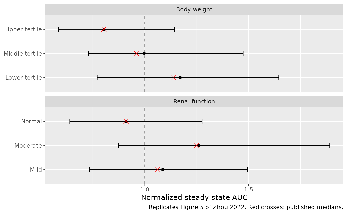
The simulated medians above carry Monte-Carlo error of about 2% (200 draws per arm with 22.7% CV on CL/F). Because the median of exp(-eta) is 1, the published medians are set by the covariate model alone, so the gate below uses the typical-value prediction at the middle of each arm’s uniform range instead; it is deterministic and holds on any machine.

fig5_mid <- fig5_arms |>
  dplyr::mutate(
    id = dplyr::row_number(),
    x = (lo + hi) / 2,
    CRCL = ifelse(cov == "CRCL", x, 90.45),
    WT = ifelse(cov == "WT", x, 65.95)
  )
fig5_typ <- rxode2::rxSolve(
  rxode2::zeroRe(mod),
  events = fig5_mid |>
    dplyr::transmute(id, time = 0, evid = 0L, amt = NA_real_, cmt = "central", CRCL, WT, arm),
  keep = "arm"
) |>
  as.data.frame() |>
  dplyr::mutate(auc_norm = 38.0 / cl) |>
  dplyr::select(arm, auc_norm) |>
  dplyr::left_join(fig5 |> dplyr::select(arm, pub_median), by = "arm") |>
  dplyr::mutate(pct_diff = 100 * (auc_norm / pub_median - 1))
#> ℹ parameter labels from comments will be replaced by 'label()'
#> ℹ omega/sigma items treated as zero: 'etalcl', 'etalmtt'
#> Warning: multi-subject simulation without without 'omega'
knitr::kable(fig5_typ, digits = 3, caption = "Typical-value normalized AUCss at each arm's mid-range covariate vs the Figure 5 median.")

Typical-value normalized AUCss at each arm’s mid-range covariate vs the Figure 5 median.
arm	auc_norm	pub_median	pct_diff
Normal	0.912	0.910	0.244
Mild	1.063	1.060	0.261
Moderate	1.255	1.250	0.376
Lower tertile	1.143	1.140	0.250
Middle tertile	0.966	0.959	0.686
Upper tertile	0.806	0.803	0.315

# Realised |pct_diff| <= 1% for all six arms. A wrong exponent (e.g. 0.484
# vs 0.325 swapped) or a wrong reference value moves at least one arm by >5%.
stopifnot(nrow(fig5_typ) == 6, all(abs(fig5_typ$pct_diff) < 3))

In the Results text the body-weight medians are listed as 0.803, 0.959 and 1.14 for the low, medium and high tertiles. Figure 5B and the Discussion (“higher TAK-931 exposures was observed with lower body weights”) put 0.803 in the upper tertile and 1.14 in the lower tertile, which is what the covariate model gives; the Results sentence has the tertile order reversed.

Assumptions and deviations

Transit-rate convention. Supplemental Figure S1 shows dose -> transit 1 -> transit 2 -> central with every transfer labelled “MTT, NTR”, and the Results state that ka was set equal to the transit rate constant. The relation between ktr and MTT is not printed. The maintainers encoded ktr = NTR / MTT = 2 / MTT, the reading that reproduces the paper’s own simulated day-1 Cmax distribution (Supplemental Table S2); the alternative ktr = (NTR + 1) / MTT = 3 / MTT overpredicts the median Cmax by about 15% and its 2.5th percentile by about 30% (see “Transit-rate convention”). AUC and trough concentrations do not discriminate between the two.
Covariate reference values. Equation 7 centres the covariates on 90.45 mL/min and 65.95 kg, which the Methods and Figure 5 call the medians of the analysis data set. Table 2 reports per-patient medians of 89.9 mL/min and 65.8 kg. The model uses the Equation 7 values.
Body weight on Vc/F. Supplemental Table S1 lists the final covariate model as “body weight on V2”, with V2 defined in that table as the peripheral volume. Equation 7, Table 3, the Results text and the Supplemental Figure S1 schema all put body weight on the central volume (V1 in Figure S1). The model follows Equation 7.
Table S2 units. Supplemental Table S2 labels AUC in ugh/mL; the values are ngh/mL (see the PKNCA section).
Virtual cohort. Body weight and creatinine clearance are drawn independently from truncated log-normal distributions matching the Table 2 medians and ranges; the paper’s simulations used the analysis data set, whose covariate joint distribution is not published. The simulated median AUC0-24 runs a few percent above Table S2, consistent with that approximation.
Trough. Table S2’s trough (“minimum concentration”) is compared with the concentration 24 h after the dose.
Figure 5 arms. For each renal-function arm body weight is held at 65.95 kg, and for each weight tertile CrCL is held at 90.45 mL/min; the paper describes the procedure for renal function and states that “the same procedure was followed” for body weight.
Residual error. The paper fits log-transformed concentrations with an additive error (SD 0.499), encoded as lnorm(expSd). All comparisons above use the individual prediction Cc without residual error, as the paper’s simulated summaries do.
Crossref lists no correction or erratum for this article as of 2026-10-03.