Desflurane uptake and disposition in piglets (Lu 2024)
Source:vignettes/articles/Lu_2024_desflurane.Rmd
Lu_2024_desflurane.RmdModel and source
Desflurane is a volatile inhalational anaesthetic with a low blood-gas partition coefficient. Lu 2024 gave seven mechanically ventilated piglets a fixed 6% inspiratory desflurane concentration for 2 h (uptake) and then 40% oxygen alone for 2 h (disposition), and followed the end-tidal gas, the femoral-arterial blood and the pulmonary-artery (mixed venous) blood concentrations. Blood concentrations were measured by headspace gas chromatography and, like the gas concentrations, are expressed as percent vapour (the partial pressure as a volume percent).
Each concentration-time curve was fitted per animal in WinNonlin with a zero-order (constant-infusion) input over the 120-min uptake phase and biexponential disposition, i.e. a two-compartment model, and Table 3 reports the mean (SD) of the individual estimates. The three sites were fitted independently, so the paper contributes three model files:
des_models <- c(
  "Lu_2024_desflurane_pig_endtidal",    # end-tidal gas
  "Lu_2024_desflurane_pig_arterial",    # femoral-arterial blood
  "Lu_2024_desflurane_pig_mixedvenous"  # pulmonary-artery (mixed venous) blood
)
site_label <- c(
  Lu_2024_desflurane_pig_endtidal = "End-tidal",
  Lu_2024_desflurane_pig_arterial = "Arterial blood",
  Lu_2024_desflurane_pig_mixedvenous = "Pulmonary artery blood"
)
mods <- lapply(stats::setNames(des_models, des_models), function(m) rxode2::rxode(readModelDb(m)))- Citation: Lu CC, Ho ST, Hu OYP, Hsiong CH, Cheng YC, Hsu CH, Lin TC (2024). Pharmacokinetics of desflurane uptake and disposition in piglets. Front Pharmacol 15:1339690. doi:10.3389/fphar.2024.1339690
- Article: Front Pharmacol 2024;15:1339690
for (m in des_models) {
  cat(m, "\n", sep = "")
  cat(strwrap(mods[[m]]$description, 76), sep = "\n")
  cat("\n\n")
}
#> Lu_2024_desflurane_pig_endtidal
#> Preclinical (pig). Two-compartment model with zero-order input for the
#> end-tidal desflurane concentration (percent vapour) in mechanically
#> ventilated piglets breathing 6 percent inspiratory desflurane for 2 h,
#> followed by a 2-h washout (Lu 2024). The compartments are those of a
#> descriptive curve fit observed in exhaled gas, not anatomical spaces. Lu
#> 2024 fitted each piglet individually in WinNonlin with constant-rate
#> (zero-order) input over the 120-min uptake phase and reported the mean of
#> the individual biexponential estimates (Table 3); the volumes and
#> clearances carried here are reconstructed from those macro-constants with
#> the clearance anchored to the printed mean, so no between-subject
#> variability or residual-error model is available and the residual SD is
#> fixed at zero. The end-tidal means are dominated by between-animal spread
#> (beta half-life 61.90 +/- 105.93 min), so this typical-value curve
#> over-predicts the observed mean end-tidal plateau by about half; prefer the
#> blood models for simulation. The input is the nominal amount of the
#> WinNonlin fit, in percent x litre: a 120-min zero-order infusion of 76.953
#> percent x litre into central corresponds to the 6 percent inspiratory
#> exposure (the amount scales only the clearance and volumes, not the
#> predicted concentrations). Lu 2024 fitted the arterial and pulmonary-artery
#> curves as separate models; see modellib('Lu_2024_desflurane_pig_arterial')
#> and modellib('Lu_2024_desflurane_pig_mixedvenous').
#>
#>
#> Lu_2024_desflurane_pig_arterial
#> Preclinical (pig). Two-compartment model with zero-order input for the
#> femoral-arterial blood desflurane concentration (percent vapour, i.e.
#> partial pressure as volume percent) in mechanically ventilated piglets
#> breathing 6 percent inspiratory desflurane for 2 h, followed by a 2-h
#> washout (Lu 2024). Lu 2024 fitted each piglet individually in WinNonlin
#> with constant-rate (zero-order) input over the 120-min uptake phase and
#> reported the mean of the individual biexponential estimates (Table 3); the
#> volumes and clearances carried here are reconstructed from those
#> macro-constants with the clearance anchored to the printed mean, so no
#> between-subject variability or residual-error model is available and the
#> residual SD is fixed at zero. The input is the nominal amount of the
#> WinNonlin fit, in percent x litre: a 120-min zero-order infusion of 53.443
#> percent x litre into central reproduces the 6 percent inspiratory exposure
#> (the amount scales only the clearance and volumes, not the predicted
#> concentrations). Lu 2024 fitted the end-tidal and pulmonary-artery curves
#> as separate models; see modellib('Lu_2024_desflurane_pig_endtidal') and
#> modellib('Lu_2024_desflurane_pig_mixedvenous').
#>
#>
#> Lu_2024_desflurane_pig_mixedvenous
#> Preclinical (pig). Two-compartment model with zero-order input for the
#> pulmonary-artery (mixed venous) blood desflurane concentration (percent
#> vapour, i.e. partial pressure as volume percent) in mechanically ventilated
#> piglets breathing 6 percent inspiratory desflurane for 2 h, followed by a
#> 2-h washout (Lu 2024). Lu 2024 fitted each piglet individually in WinNonlin
#> with constant-rate (zero-order) input over the 120-min uptake phase and
#> reported the mean of the individual biexponential estimates (Table 3); the
#> volumes and clearances carried here are reconstructed from those
#> macro-constants with the clearance anchored to the printed mean, so no
#> between-subject variability or residual-error model is available and the
#> residual SD is fixed at zero. The input is the nominal amount of the
#> WinNonlin fit, in percent x litre: a 120-min zero-order infusion of 52.291
#> percent x litre into central reproduces the 6 percent inspiratory exposure
#> (the amount scales only the clearance and volumes, not the predicted
#> concentrations). Lu 2024 fitted the end-tidal and femoral-arterial curves
#> as separate models; see modellib('Lu_2024_desflurane_pig_endtidal') and
#> modellib('Lu_2024_desflurane_pig_arterial').
Population
Seven male domestic piglets, 5 months old and weighing 28 +/- 5 kg, were anaesthetised with intramuscular tiletamine/zolazepam and atropine, maintained on fentanyl, propofol and pancuronium, tracheostomised and ventilated with 40% oxygen at a tidal volume of 8 mL/kg (Lu 2024 Sections 2.2-2.3). Desflurane was delivered through a vaporiser at a 5 L/min fresh-gas flow. Arterial and pulmonary-artery blood was drawn simultaneously at 1, 3, 5, 10, 20, 30, 40, 50, 60, 80, 100 and 120 min of each phase (Section 2.5). End-tidal values below 0.2% were discarded, which truncates the end-tidal curve after about 60 min of washout (Sections 2.4 and 4.5). No covariates were investigated.
str(mods[["Lu_2024_desflurane_pig_arterial"]]$population)
#> List of 10
#>  $ species       : chr "pig (domestic piglets)"
#>  $ n_subjects    : num 7
#>  $ n_studies     : num 1
#>  $ age_range     : chr "5 months"
#>  $ weight_mean   : chr "28 +/- 5 kg"
#>  $ sex_female_pct: num 0
#>  $ disease_state : chr "Healthy piglets under general anaesthesia (tiletamine/zolazepam and atropine induction; fentanyl, propofol and "| __truncated__
#>  $ dose_range    : chr "Desflurane 6 percent inspiratory via a 5 L/min fresh-gas flow for 120 min (uptake), then 40 percent oxygen alon"| __truncated__
#>  $ regions       : chr "Taiwan"
#>  $ notes         : chr "Lu 2024 Sections 2.2-2.5: seven male domestic piglets, fasted overnight. Femoral-arterial and pulmonary-artery "| __truncated__
Source trace
Every ini() value carries its origin as an in-file
comment; the table below collects them.
| Equation / parameter | Value | Source location |
|---|---|---|
Disposition equation
Y = A*exp(-alpha*t) + B*exp(-beta*t)
|
n/a | Table 3 footnote |
| Zero-order input over the 120-min uptake phase | n/a | Abstract; Section 4.2; Figure 3 caption |
Lu_2024_desflurane_pig_endtidal |
||
lcl |
0.07 L/min | Table 3, end-tidal, Clearance |
lvc |
0.10474 L | derived CL/k10 from Table 3 end-tidal A, B, alpha and
beta half-lives (Table 3 prints 0.10) |
lq |
0.026351 L/min | derived k12*vc, Table 3 end-tidal macro-constants |
lvp |
1.7017 L | derived q/k21, Table 3 end-tidal macro-constants |
Lu_2024_desflurane_pig_arterial |
||
lcl |
0.08 L/min | Table 3, arterial blood, Clearance |
lvc |
0.10349 L | derived CL/k10 from Table 3 arterial A, B, alpha and
beta half-lives (Table 3 prints 1.09; see below) |
lq |
0.020623 L/min | derived k12*vc, Table 3 arterial macro-constants |
lvp |
1.0929 L | derived q/k21, Table 3 arterial macro-constants |
Lu_2024_desflurane_pig_mixedvenous |
||
lcl |
0.09 L/min | Table 3, pulmonary artery blood, Clearance |
lvc |
0.34996 L | derived CL/k10 from Table 3 pulmonary artery A, B,
alpha and beta half-lives (Table 3 prints 0.35) |
lq |
0.038638 L/min | derived k12*vc, Table 3 pulmonary artery
macro-constants |
lvp |
2.3577 L | derived q/k21, Table 3 pulmonary artery
macro-constants |
addSd (all three files) |
0 (fixed) | not reported; see Assumptions |
Reconstructing the parameters from Table 3
Table 3 gives the biexponential macro-constants (A, B and the alpha and beta half-lives) together with secondary parameters (clearance, central volume, steady-state volume, mean residence time). The rate constants follow from the macro-constants alone; the clearance then fixes the scale of the volumes. The chunk below repeats the derivation from the Table 3 means and, in the other direction, recovers the macro-constants from the packaged parameters.
tab3 <- data.frame(
  model = des_models,
  A = c(731.26, 514.32, 147.32),       # %, Table 3
  B = c(3.45, 2.11, 2.10),             # %, Table 3
  thalpha = c(0.75, 0.71, 1.86),       # min, Table 3
  thbeta = c(61.90, 46.39, 61.29),     # min, Table 3
  CL = c(0.07, 0.08, 0.09),            # L/min, Table 3
  Vc = c(0.10, 1.09, 0.35),            # L, Table 3
  Vss = c(1.29, 1.20, 2.75),           # L, Table 3
  MRT = c(15.51, 15.00, 31.26),        # min, Table 3
  cmax = c(5.68, 4.85, 4.07),          # %, Table 3
  aucinf.obs = c(695.88, 603.03, 533.10) # % x min, Table 3
)

# Packaged typical values, read back from each model file
pk <- bind_rows(lapply(des_models, function(m) {
  th <- mods[[m]]$theta
  data.frame(
    model = m,
    cl = exp(th[["lcl"]]), vc = exp(th[["lvc"]]),
    q = exp(th[["lq"]]), vp = exp(th[["lvp"]])
  )
}))

recovered <- pk |>
  mutate(
    k10 = cl / vc, k12 = q / vc, k21 = q / vp,
    s = k10 + k12 + k21, p = k10 * k21,
    alpha = (s + sqrt(s^2 - 4 * p)) / 2,
    beta = (s - sqrt(s^2 - 4 * p)) / 2
  ) |>
  left_join(tab3, by = "model") |>
  mutate(
    # nominal input amount implied by the fit: A + B = dose / vc
    dose = vc * (A + B),
    A_rec = dose / vc * (alpha - k21) / (alpha - beta),
    B_rec = dose / vc * (k21 - beta) / (alpha - beta),
    thalpha_rec = log(2) / alpha,
    thbeta_rec = log(2) / beta,
    Vss_rec = vc + vp,
    MRT_rec = Vss_rec / cl,
    # central volume implied by the PRINTED Vss and MRT with the macro-constants
    Vc_check = Vss * (A / (log(2) / thalpha) + B / (log(2) / thbeta)) / ((A + B) * MRT)
  )

recovered |>
  transmute(
    Site = site_label[model],
    A = sprintf("%.2f / %.2f", A, A_rec),
    B = sprintf("%.2f / %.2f", B, B_rec),
    `alpha t1/2 (min)` = sprintf("%.2f / %.2f", thalpha, thalpha_rec),
    `beta t1/2 (min)` = sprintf("%.2f / %.2f", thbeta, thbeta_rec),
    `Input amount (% x L)` = sprintf("%.3f", dose)
  ) |>
knitr::kable(caption = "Table 3 macro-constants (printed / recovered from the packaged model).")| Site | A | B | alpha t1/2 (min) | beta t1/2 (min) | Input amount (% x L) |
|---|---|---|---|---|---|
| End-tidal | 731.26 / 731.26 | 3.45 / 3.45 | 0.75 / 0.75 | 61.90 / 61.90 | 76.953 |
| Arterial blood | 514.32 / 514.32 | 2.11 / 2.11 | 0.71 / 0.71 | 46.39 / 46.39 | 53.443 |
| Pulmonary artery blood | 147.32 / 147.32 | 2.10 / 2.10 | 1.86 / 1.86 | 61.29 / 61.29 | 52.291 |
stopifnot(
  # Closed-form round trip on the same numbers: only floating-point error.
  all(abs(recovered$A_rec / recovered$A - 1) < 1e-5),
  all(abs(recovered$B_rec / recovered$B - 1) < 1e-5),
  all(abs(recovered$thalpha_rec / recovered$thalpha - 1) < 1e-5),
  all(abs(recovered$thbeta_rec / recovered$thbeta - 1) < 1e-5)
)
The secondary parameters Table 3 prints act as an external check, because they were averaged across animals separately from the macro-constants:
recovered |>
  transmute(
    Site = site_label[model],
    `CL (L/min) printed / packaged` = sprintf("%.2f / %.3f", CL, cl),
    `Vc (L) printed / packaged` = sprintf("%.2f / %.3f", Vc, vc),
    `Vss (L) printed / packaged` = sprintf("%.2f / %.3f", Vss, Vss_rec),
    `MRT (min) printed / packaged` = sprintf("%.2f / %.2f", MRT, MRT_rec)
  ) |>
knitr::kable(caption = "Table 3 secondary parameters against the packaged models.")| Site | CL (L/min) printed / packaged | Vc (L) printed / packaged | Vss (L) printed / packaged | MRT (min) printed / packaged |
|---|---|---|---|---|
| End-tidal | 0.07 / 0.070 | 0.10 / 0.105 | 1.29 / 1.806 | 15.51 / 25.81 |
| Arterial blood | 0.08 / 0.080 | 1.09 / 0.103 | 1.20 / 1.196 | 15.00 / 14.96 |
| Pulmonary artery blood | 0.09 / 0.090 | 0.35 / 0.350 | 2.75 / 2.708 | 31.26 / 30.09 |
For the two blood sites the packaged parameters regenerate the
printed steady-state volumes and mean residence times to within 4%, and
the pulmonary-artery central volume to rounding. The arterial
central volume is printed as 1.09 L, but with the arterial
macro-constants the central volume is fixed at
Vss * AUC / ((A + B) * MRT) = 0.103 L from the printed Vss
and MRT, whatever the input amount, and 1.09 L is instead the derived
peripheral volume (1.093 L = Vss - Vc). The packaged arterial
model therefore uses the central volume implied by the macro-constants;
the printed 1.09 L is treated as a transcription slip.
The end-tidal means do not hang together as one curve: the beta half-life is 61.90 +/- 105.93 min, so the mean is pulled by one or more animals with a long terminal phase, and the reconstructed Vss and MRT exceed the printed means by 40-65%. The model reproduces the printed end-tidal macro-constants exactly, but, as the comparisons below show, a curve built from those mean macro-constants over-predicts the observed end-tidal plateau.
The product CL x AUC is close to 48 % x L for all three
sites (0.07 x 695.88, 0.08 x 603.03, 0.09 x 533.10), which suggests the
fits used one nominal input amount. The packaged models instead take the
amount implied by each site’s printed clearance (the “Input amount”
column above). Because the amount and the volumes scale together, this
choice changes the clearance and volumes but not the predicted
concentrations.
Simulation
The 6% inspiratory exposure is a zero-order infusion of each model’s
nominal input amount into central over 120 min, followed by
120 min of washout. The models have no between-subject variability, so a
single typical-value profile per site is the model prediction.
obs_times <- sort(unique(c(seq(0, 240, by = 0.5), 121, 123, 125, 130, 140, 180)))

sim <- bind_rows(lapply(des_models, function(m) {
  d <- recovered$dose[recovered$model == m]
  ev <- rxode2::et(amt = d, dur = 120, cmt = "central") |>
    rxode2::et(obs_times)
  out <- rxode2::rxSolve(mods[[m]], ev, returnType = "data.frame")
  out$model <- m
  out
}))
sim$site <- factor(site_label[sim$model], levels = site_label)
Replicate Figure 3
Table 1 reports the observed mean (SD) at 1, 3, 5, 10, 20, 60 and 120 min of each phase; Figure 3 shows the same means against the fitted curves.
t1_times <- c(1, 3, 5, 10, 20, 60, 120)
table1 <- data.frame(
  site = rep(site_label, each = 14),
  time = rep(c(t1_times, 120 + t1_times), 3),
  mean = c(
    # End-tidal (ET), %; '--' at 120 min of disposition (below the 0.2% cutoff)
    3.39, 4.75, 4.93, 5.35, 5.45, 5.61, 5.76, 2.18, 1.23, 1.04, 0.64, 0.38, 0.20, NA,
    # Arterial blood (A), %
    2.75, 3.65, 4.00, 4.17, 4.44, 4.58, 4.65, 2.23, 1.39, 1.24, 0.84, 0.54, 0.32, 0.23,
    # Pulmonary artery blood (PA), %
    1.15, 2.24, 2.61, 3.02, 3.27, 3.62, 4.10, 2.96, 2.08, 1.69, 1.22, 0.85, 0.49, 0.34
  ),
  sd = c(
    0.79, 0.62, 0.23, 0.28, 0.09, 0.09, 0.05, 0.88, 0.47, 0.55, 0.17, 0.10, 0.04, NA,
    0.67, 0.39, 0.53, 0.54, 0.39, 0.40, 0.26, 0.87, 0.43, 0.47, 0.17, 0.07, 0.05, 0.06,
    0.65, 0.45, 0.39, 0.26, 0.34, 0.47, 0.41, 0.54, 0.39, 0.33, 0.23, 0.13, 0.06, 0.05
  )
) |>
  filter(!is.na(mean))
table1$site <- factor(table1$site, levels = site_label)
ggplot(sim, aes(time, Cc)) +
  geom_line(colour = "steelblue") +
  geom_pointrange(
    data = table1,
    aes(time, mean, ymin = mean - sd, ymax = mean + sd),
    shape = 1, size = 0.3
  ) +
  facet_wrap(~site, ncol = 1) +
  scale_x_continuous(breaks = seq(0, 240, by = 60)) +
  labs(x = "Time (min)", y = "Desflurane concentration (%)")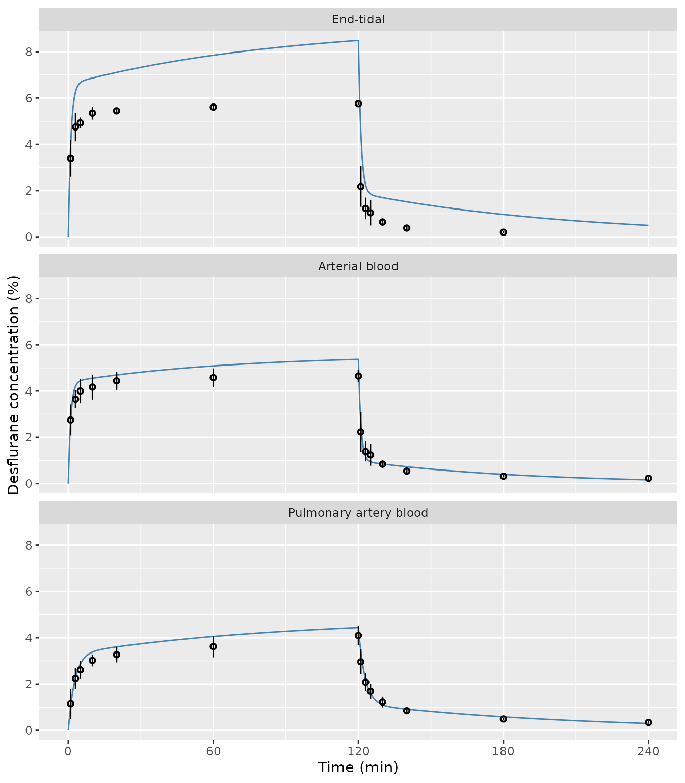
Replicates Figure 3 of Lu 2024: typical-value prediction from the mean Table 3 parameters (line) against the observed means +/- SD from Table 1 (points).
cmp <- table1 |>
  left_join(sim |> select(site, time, Cc), by = c("site", "time")) |>
  mutate(pct_diff = 100 * (Cc - mean) / mean)

cmp |>
  mutate(
    Phase = if_else(time <= 120, "uptake", "disposition"),
    `Phase time (min)` = if_else(time <= 120, time, time - 120)
  ) |>
  select(site, Phase, `Phase time (min)`, mean, Cc, pct_diff) |>
  mutate(Cc = signif(Cc, 3), pct_diff = round(pct_diff, 1)) |>
  rename(
    "Site" = site,
    "Observed mean (%)" = mean,
    "Model (%)" = Cc,
    "Difference (%)" = pct_diff
  ) |>
knitr::kable(caption = "Model prediction against the Table 1 means.")| Site | Phase | Phase time (min) | Observed mean (%) | Model (%) | Difference (%) |
|---|---|---|---|---|---|
| End-tidal | uptake | 1 | 3.39 | 4.010 | 18.2 |
| End-tidal | uptake | 3 | 4.75 | 6.270 | 31.9 |
| End-tidal | uptake | 5 | 4.93 | 6.670 | 35.3 |
| End-tidal | uptake | 10 | 5.35 | 6.870 | 28.3 |
| End-tidal | uptake | 20 | 5.45 | 7.110 | 30.4 |
| End-tidal | uptake | 60 | 5.61 | 7.850 | 39.9 |
| End-tidal | uptake | 120 | 5.76 | 8.490 | 47.4 |
| End-tidal | disposition | 1 | 2.18 | 4.490 | 106.1 |
| End-tidal | disposition | 3 | 1.23 | 2.250 | 82.7 |
| End-tidal | disposition | 5 | 1.04 | 1.860 | 78.8 |
| End-tidal | disposition | 10 | 0.64 | 1.700 | 165.2 |
| End-tidal | disposition | 20 | 0.38 | 1.520 | 299.2 |
| End-tidal | disposition | 60 | 0.20 | 0.969 | 384.6 |
| Arterial blood | uptake | 1 | 2.75 | 2.750 | 0.1 |
| Arterial blood | uptake | 3 | 3.65 | 4.210 | 15.3 |
| Arterial blood | uptake | 5 | 4.00 | 4.440 | 11.0 |
| Arterial blood | uptake | 10 | 4.17 | 4.550 | 9.2 |
| Arterial blood | uptake | 20 | 4.44 | 4.690 | 5.7 |
| Arterial blood | uptake | 60 | 4.58 | 5.090 | 11.1 |
| Arterial blood | uptake | 120 | 4.65 | 5.370 | 15.5 |
| Arterial blood | disposition | 1 | 2.23 | 2.620 | 17.5 |
| Arterial blood | disposition | 3 | 1.39 | 1.170 | -15.6 |
| Arterial blood | disposition | 5 | 1.24 | 0.944 | -23.9 |
| Arterial blood | disposition | 10 | 0.84 | 0.845 | 0.6 |
| Arterial blood | disposition | 20 | 0.54 | 0.728 | 34.7 |
| Arterial blood | disposition | 60 | 0.32 | 0.400 | 25.1 |
| Arterial blood | disposition | 120 | 0.23 | 0.163 | -29.0 |
| Pulmonary artery blood | uptake | 1 | 1.15 | 1.040 | -9.4 |
| Pulmonary artery blood | uptake | 3 | 2.24 | 2.270 | 1.3 |
| Pulmonary artery blood | uptake | 5 | 2.61 | 2.870 | 9.9 |
| Pulmonary artery blood | uptake | 10 | 3.02 | 3.380 | 11.9 |
| Pulmonary artery blood | uptake | 20 | 3.27 | 3.610 | 10.3 |
| Pulmonary artery blood | uptake | 60 | 3.62 | 4.060 | 12.1 |
| Pulmonary artery blood | uptake | 120 | 4.10 | 4.440 | 8.4 |
| Pulmonary artery blood | disposition | 1 | 2.96 | 3.410 | 15.1 |
| Pulmonary artery blood | disposition | 3 | 2.08 | 2.190 | 5.2 |
| Pulmonary artery blood | disposition | 5 | 1.69 | 1.600 | -5.5 |
| Pulmonary artery blood | disposition | 10 | 1.22 | 1.110 | -9.4 |
| Pulmonary artery blood | disposition | 20 | 0.85 | 0.918 | 8.0 |
| Pulmonary artery blood | disposition | 60 | 0.49 | 0.583 | 19.0 |
| Pulmonary artery blood | disposition | 120 | 0.34 | 0.296 | -13.0 |
The pulmonary-artery curve tracks the observed means through both phases to within about 15%. The arterial curve runs 5-15% high on the uptake plateau and is up to about 30% off the observed means during washout, where the fast alpha phase (half-life 0.71 min) makes the early disposition points sensitive to averaging across animals. The end-tidal curve reaches a plateau far above the 6% inspired concentration, which is physically impossible for an end-tidal value. This is the averaging artefact described above, not a property of the measured data.
blood <- cmp |> filter(site != "End-tidal")
stopifnot(
  # Uptake plateau (20-120 min): the blood models sit within ~15% of the
  # observed means. The prediction is deterministic (no random effects).
  all(abs(blood$pct_diff[blood$time %in% c(20, 60, 120)]) < 20),
  # Across all tabulated blood timepoints the centre of the error is modest.
  abs(median(blood$pct_diff)) < 15
)
Validation against the published NCA (PKNCA)
Table 3 reports Cmax and AUC for each site. In a WinNonlin infusion
fit the AUC is the area under the fitted curve to infinity, so it is
compared with PKNCA’s aucinf.obs on the simulated
profile.
conc <- sim |>
  filter(!is.na(Cc)) |>
  mutate(id = 1L, treatment = as.character(site)) |>
  select(id, treatment, time, Cc)

dose_df <- recovered |>
  transmute(id = 1L, treatment = site_label[model], time = 0, amt = dose, duration = 120)

conc_obj <- PKNCA::PKNCAconc(conc, Cc ~ time | treatment + id)
dose_obj <- PKNCA::PKNCAdose(
  dose_df, amt ~ time | treatment + id,
  duration = "duration", route = "intravascular"
)
intervals <- data.frame(start = 0, end = Inf, cmax = TRUE, tmax = TRUE, aucinf.obs = TRUE)
nca_res <- PKNCA::pk.nca(PKNCA::PKNCAdata(conc_obj, dose_obj, intervals = intervals))

reference <- tab3 |>
  transmute(treatment = site_label[model], cmax, aucinf.obs)

nca_tbl <- nlmixr2lib::ncaComparisonTable(
  nca_res, reference,
  by = "treatment",
  params = c("cmax", "aucinf.obs"),
  units = c(cmax = "%", aucinf.obs = "% x min")
)
nca_tbl |>
  dplyr::rename("Site" = treatment) |>
knitr::kable(caption = "Simulated NCA against Lu 2024 Table 3.")| NCA parameter | Site | Reference | Simulated | % diff |
|---|---|---|---|---|
| Cmax (%) | End-tidal | 5.68 | 8.49 | +49.5%* |
| Cmax (%) | Arterial blood | 4.85 | 5.37 | +10.7% |
| Cmax (%) | Pulmonary artery blood | 4.07 | 4.44 | +9.2% |
| AUC0-∞ (obs) (% x min) | End-tidal | 696 | 1100 | +58.0%* |
| AUC0-∞ (obs) (% x min) | Arterial blood | 603 | 668 | +10.8% |
| AUC0-∞ (obs) (% x min) | Pulmonary artery blood | 533 | 581 | +9.0% |
- differs from reference by more than ±20%.
The two blood models reproduce the printed Cmax and AUC within about 11%; the residual is the expected gap between a curve built from mean parameters and the mean of the individual Cmax and AUC values. The end-tidal row is starred for the reason given above.
nca_wide <- as.data.frame(nca_res) |>
  select(treatment, PPTESTCD, PPORRES) |>
  pivot_wider(names_from = PPTESTCD, values_from = PPORRES) |>
  left_join(reference, by = "treatment", suffix = c("_sim", "_ref")) |>
  filter(treatment != "End-tidal")
stopifnot(
  all(abs(nca_wide$cmax_sim / nca_wide$cmax_ref - 1) < 0.15),
  all(abs(nca_wide$aucinf.obs_sim / nca_wide$aucinf.obs_ref - 1) < 0.15)
)
Assumptions and deviations
- Typical values only. Lu 2024 fitted each piglet separately and reported the mean and SD of the individual estimates; there is no population model, so the packaged models carry no between-subject variability and the residual SD is fixed at zero.
- Parameterisation. The volumes and intercompartmental clearance are derived from the Table 3 macro-constants, with the clearance anchored to the printed Table 3 mean. Any other anchor would rescale the volumes and the input amount together without changing the predicted concentrations.
- Input amount. The paper does not state the dose amount used in the WinNonlin fits. Each model’s description gives the amount, in % x L, that the packaged clearance implies for the 6%, 120-min exposure. Simulating other inspired concentrations by scaling the infusion rate in proportion assumes the linear zero-order input the authors fitted; the paper studied 6% only.
- Arterial central volume. The printed 1.09 L is inconsistent with the arterial macro-constants and equals the derived peripheral volume; the model uses the 0.103 L the macro-constants imply.
-
End-tidal model. Shipped for completeness. Its mean
macro-constants over-predict the observed end-tidal plateau by about 50%
and should not be used for quantitative end-tidal simulation. The
compartmentDataspecimen for its states is “not applicable”, because they are curve-fit spaces observed through exhaled gas, for which the specimen vocabulary has no member. - Concentration units. All concentrations are percent vapour (the partial pressure as a volume percent), as reported. Converting blood values to an amount requires the blood-gas partition coefficient (0.38 +/- 0.01 in these piglets).