Cefazolin (Bausch 2024)
Source:vignettes/articles/Bausch_2024_cefazolin.Rmd
Bausch_2024_cefazolin.RmdModel and source
- Citation: Bausch S, Draeger S, Charitos-Fragkakis P, Egli A, Moser S, Hinic V, Kuehl R, Bassetti S, Siegemund M, Rentsch KM, Hermann L, Schoening V, Hammann F, Sendi P, Osthoff M. Target Attainment and Population Pharmacokinetics of Cefazolin in Patients with Invasive Staphylococcus aureus Infections: A Prospective Cohort Study. Antibiotics (Basel). 2024;13(10):928. doi:10.3390/antibiotics13100928. PMCID PMC11504871. Binding equations from the Results Sect. 2.5 display equation; all parameter estimates and covariate relationships from Supplementary Table S2; model-building sequence from Supplementary Table S3.
- Description: One-compartment joint total/unbound population PK model for intravenous cefazolin in adults with invasive Staphylococcus aureus infection (Bausch 2024). The disposition is carried on the UNBOUND concentration Cu = central/V with linear unbound clearance; the measured TOTAL plasma concentration is reconstructed as Cc = Cu + Cb, where the bound concentration Cb = Bmax * Cu / (kd + Cu) + NS * Cu combines a saturable albumin-binding site with a linear non-saturable component. Total and unbound concentrations are BOTH observed endpoints, each with its own proportional residual error. Clearance carries an allometric Cockcroft-Gault creatinine-clearance term, volume an allometric weight term with the exponent FIXED at 1, and the non-saturable binding constant an allometric serum-albumin term. Inter-individual variability on V and Bmax; inter-occasion variability on CL and NS across the four therapeutic-drug-monitoring sampling days.
- Article: https://doi.org/10.3390/antibiotics13100928
- Supplement (Tables S1-S3, Figures S1-S6): https://www.mdpi.com/2079-6382/13/10/928/s1
Population
Bausch 2024 is a single-centre prospective observational cohort and PK/PD study run at the University Hospital Basel between January 2020 and December 2021 (ClinicalTrials.gov NCT04503252). Fifty-one adults with invasive methicillin-susceptible Staphylococcus aureus infection contributed 226 paired total and unbound cefazolin plasma concentrations, a mean of 4.4 per patient (Table 1, Table 2). The cohort is elderly (median age 74.1 years, IQR 56.6-81.8), predominantly male (25.5% female), of median weight 73 kg (IQR 67-93) and median BMI 24.5 kg/m^2 – so the model was not fitted in an obese population. Three quarters (76.5%) had bloodstream infection; endocarditis and osteomyelitis or septic arthritis each accounted for 19.6%.
Two features of the population are load-bearing for the model. First it is hypoalbuminaemic: median serum albumin was 29.0 g/L at onset of infection (Table 1) and 25 g/L at the first drug measurement (Table S1), well below a healthy 35-50 g/L, and the weighted mean albumin the model centres on is lower still at 24.0844 g/L. Second, renal function spans a wide range – median eGFR (CKD-EPI) 76 mL/min/1.73 m^2 with IQR 41-91, chronic kidney disease stage G3 in 9.8% and G4 in 9.8%, and acute kidney injury in 11.8%. Haemodialysis was an exclusion criterion and no patient required renal replacement therapy during the study, so the model carries no information about dialysis.
The paper’s central observation is that the unbound fraction is both higher and far more variable than the 20% conventionally assumed: mean 27.0% (SD 13.4), ranging from 8.9% to 79.7%, and correlated with both albumin (r = 0.58) and eGFR (r = -0.42). That variability is what the saturable-binding model below exists to describe.
The same information is available programmatically via the model’s
population metadata
(readModelDb("Bausch_2024_cefazolin")()$population).
Model structure
The authors compared one-, two- and three-compartment structural models with linear, zero-order and Michaelis-Menten elimination, and four different protein-binding parameterisations (Supplementary Table S3). The winning model is a one-compartment joint model of total and unbound concentration whose binding equation is given in Results Sect. 2.5:
Both endpoints are measured, and each carries its own proportional residual error.
Two encoding decisions deserve to be stated explicitly, because the paper prints the binding equations without saying how they couple to the PK.
The disposition is carried on the unbound
concentration. The equations above compute Cbound
from Cunbound, so the state that the ODE
integrates must be the one that yields Cunbound. This is
also the only reading consistent with the magnitudes: Table S2 reports
CL = 15.6 L/h and V = 67.2 L, whereas total-referenced cefazolin values
are roughly 4 L/h and 10 L, i.e. both are inflated by about the
reciprocal of the reported 27% unbound fraction. The verification
section below confirms it against the paper’s own observed concentration
medians.
A consequence worth flagging for anyone reusing the model: because
clearance is unbound-referenced, the unbound concentration is
independent of the binding parameters. Albumin moves
the total concentration and hence the unbound fraction, but it
does not move unbound exposure. That is the standard result for
a renally cleared drug with unbound-referenced clearance, and it is
internally consistent with the paper, which retains albumin on
NS alone.
Albumin acts on NS, not on
kd. The Table S2 legend glosses
Albumin_NS as the “exponent for the allometrically scaled
albumin on kd”, but the Covariate Relationships block of that same table
heads its third row NS and prints
NS_pop * (Albumin/Albumin_mean)^Albumin_NS; and Table S3’s
winning row in the final binding block is “GFR-CG on Cl / Albumin on NS
/ Weight on Vd” at OFV 2816.93, better than the “Albumin on kd”
alternative at 2854.78. The legend gloss is a leftover from the kd-only
variant the authors tried and rejected. The model follows the equation
and the model-building table.
Source trace
The per-parameter origin is recorded as an in-file comment next to
each ini() entry in
inst/modeldb/specificDrugs/Bausch_2024_cefazolin.R. The
table below collects them in one place for review. Every value comes
from the Supplementary Table S2 “Final joint model” column except where
noted.
| Equation / parameter | Value | Source location |
|---|---|---|
lcl (CL) |
15.6 L/h | Table S2, CL_pop [3.8% RSE]; bootstrap 13.4-19.1 |
lvc (V) |
67.2 L | Table S2, V_pop [7.3% RSE]; bootstrap 55.7-90.1 |
lbmax_pb (Bmax) |
55.2 mg/L | Table S2, Bmax_pop [10.7% RSE]; bootstrap
33.5-80.1 |
lkd_pb (kd) |
12.7 mg/L | Table S2, kd_pop [10.1% RSE]; bootstrap 7.1-21.2 |
lns_pb (NS) |
0.5 | Table S2, NS_pop [18.6% RSE]; bootstrap 0.4-1.0 |
e_crcl_cl |
1.2 | Table S2, GFR_CL [5.0% RSE]; bootstrap 0.9-1.4 |
e_wt_vc |
1.0 (fixed) | Table S2, Weight_V (fixed); no RSE, bootstrap n/a |
e_alb_ns |
2.4 | Table S2, Albumin_NS [12.0% RSE]; bootstrap
1.8-3.9 |
| CRCL reference | 80.1634 mL/min | Table S2 legend, GFR_mean (weighted mean eGFR-CG) |
| WT reference | 70 kg | Table S2 Covariate Relationships, literal denominator of the V equation |
| ALB reference | 24.0844 g/L | Table S2 legend, Albumin_mean (weighted mean
albumin) |
etalvc |
0.16 (= 0.4^2) | Table S2, V_IIV = 0.4 [15.6% RSE] (Monolix SD) |
etalbmax_pb |
0.04 (= 0.2^2) | Table S2, Bmax_IIV = 0.2 [21.0% RSE] (Monolix SD) |
etaiov_cl_* |
0.16 (= 0.4^2) | Table S2, CL_IOV = 0.4 [7.12% RSE] (Monolix SD) |
etaiov_ns_* |
0.04 (= 0.2^2) | Table S2, NS_IOV = 0.2 [31.0% RSE] (Monolix SD) |
propSd (total) |
0.2 | Table S2, Residual error, Proportional (b), Total [8.33% RSE] |
propSd_Cu (unbound) |
0.2 | Table S2, Residual error, Proportional (b), Unbound [7.79% RSE] |
| Binding equation | n/a | Results Sect. 2.5 display equation |
CL = CL_pop * (GFR/GFR_mean)^GFR_CL |
n/a | Table S2, Covariate Relationships, row CL
|
V = V_pop * (Weight/70)^Weight_V |
n/a | Table S2, Covariate Relationships, row V
|
NS = NS_pop * (Albumin/Albumin_mean)^Albumin_NS |
n/a | Table S2, Covariate Relationships, row NS
|
| 4 IOV occasions | n/a | Methods Sect. 4.4 / Figure S6 sampling days 1, 3, 7, 14 |
Verification against the paper’s observed concentrations
Bausch 2024 reports no NCA parameters, so the strongest available check on the transcription is the paper’s own Table 2: median measured mid-dose and trough concentrations, for both the total and the unbound analyte, on study day 1. Four independent numbers, two of them on an endpoint (total) that depends on the whole binding isotherm.
The typical patient is simulated at the model’s own centring covariates (eGFR-CG 80.1634 mL/min, 70 kg, albumin 24.0844 g/L) on the protocol regimen of 2 g every 8 h as a 30-minute infusion, run to steady state. “Mid-dose” is the paper’s definition: after 50% of the dosing interval (Methods Sect. 4.4).
mod <- readModelDb("Bausch_2024_cefazolin")
mod_typical <- rxode2::zeroRe(mod)
#> ℹ parameter labels from comments will be replaced by 'label()'
#> Warning: some etas defaulted to non-mu referenced, possible parsing error: etaiov_cl_1, etaiov_cl_2, etaiov_cl_3, etaiov_cl_4, etaiov_ns_1, etaiov_ns_2, etaiov_ns_3, etaiov_ns_4
#> as a work-around try putting the mu-referenced expression on a simple line
#> Warning: some etas defaulted to non-mu referenced, possible parsing error: etaiov_cl_1, etaiov_cl_2, etaiov_cl_3, etaiov_cl_4, etaiov_ns_1, etaiov_ns_2, etaiov_ns_3, etaiov_ns_4
#> as a work-around try putting the mu-referenced expression on a simple line

# Steady state on 2 g q8h, 30-minute infusion. The model declares two
# endpoints (Cc and Cu), so observation rows must nominate one -- done here
# with `dvid` (dvid 1 = Cc, dvid 2 = Cu), which is the documented multi-output
# mechanism. Doses go to the ODE state `central`; both Cc and Cu come back as
# columns regardless of which endpoint a row nominates.
ev_typ <- rxode2::et(amt = 2000, dur = 0.5, cmt = "central", ii = 8, until = 240) |>
  rxode2::et(seq(240, 248, by = 0.05)) |>
  as.data.frame() |>
  dplyr::mutate(CRCL = 80.1634, WT = 70, ALB = 24.0844, OCC = 1,
                dvid = ifelse(evid == 0, 1L, NA_integer_))

sim_typ <- rxode2::rxSolve(mod_typical, ev_typ, omega = NA, sigma = NA,
                           returnType = "data.frame") |>
  dplyr::filter(time >= 240) |>
  dplyr::mutate(tad = time - 240)

# Trough = end of the interval; mid-dose = 50% of the interval (4 h).
pick <- function(d, tad_want) d[which.min(abs(d$tad - tad_want)), ]
tr <- pick(sim_typ, 8)
md <- pick(sim_typ, 4)

chk <- tibble::tribble(
  ~analyte,  ~timepoint,  ~simulated,  ~published,
  "Total",   "Mid-dose",  md$Cc,       51.6,
  "Total",   "Trough",    tr$Cc,       26.4,
  "Unbound", "Mid-dose",  md$Cu,       12.1,
  "Unbound", "Trough",    tr$Cu,       5.4
) |>
  dplyr::mutate(pct_diff = 100 * (simulated - published) / published)

chk |>
  dplyr::mutate(dplyr::across(c(simulated, published, pct_diff), \(x) round(x, 1))) |>
  dplyr::rename(
    "Analyte"                = analyte,
    "Timepoint"              = timepoint,
    "Simulated (mg/L)"       = simulated,
    "Bausch 2024 Table 2 median (mg/L)" = published,
    "Difference (%)"         = pct_diff
  ) |>
  knitr::kable(
    caption = "Typical-value steady-state concentrations vs the observed medians of Bausch 2024 Table 2 (study day 1, 2 g q8h).",
    align = c("l", "l", "r", "r", "r")
)| Analyte | Timepoint | Simulated (mg/L) | Bausch 2024 Table 2 median (mg/L) | Difference (%) |
|---|---|---|---|---|
| Total | Mid-dose | 51.8 | 51.6 | 0.5 |
| Total | Trough | 26.1 | 26.4 | -1.0 |
| Unbound | Mid-dose | 14.8 | 12.1 | 22.1 |
| Unbound | Trough | 5.8 | 5.4 | 8.1 |
Both total concentrations land within 1% of the
published medians, and the unbound values within 8% (trough) and 22%
(mid-dose). That the total endpoint – which depends on
Bmax, kd, NS and the albumin
exponent as well as on CL and V – reproduces
to within 1% at two different points of the dosing interval is what
confirms the structural reading and the parameter transcription
together. The looser agreement on unbound mid-dose is expected:
“mid-dose” is a nominal sampling time in a clinical cohort where the
true time after dose varies, some patients were dosed every 6 h rather
than every 8 h, and the comparison is a simulated typical value against
an observed cohort median.
This check is deterministic (random effects zeroed, no residual error), so it is gated tightly.
# Deterministic comparison -- no RNG involved, so an exact-ish bound is correct
# here and must NOT be loosened. The two total-concentration rows are the
# structural gate; the unbound rows are gated more loosely for the
# nominal-sampling-time reason given above.
stopifnot(
  all(abs(chk$pct_diff[chk$analyte == "Total"]) < 5),
  all(abs(chk$pct_diff[chk$analyte == "Unbound"]) < 30)
)

# The unbound fraction the model produces must sit inside the range the paper
# reports for the cohort (mean 27.0%, SD 13.4, observed 8.9%-79.7%).
fu_sim <- 100 * c(md$Cu / md$Cc, tr$Cu / tr$Cc)
stopifnot(all(fu_sim > 8.9), all(fu_sim < 79.7))
round(fu_sim, 1)
#> [1] 28.5 22.3
PKNCA validation
With no published NCA table to compare against, the NCA is used to check the model against its own closed-form identities, which is the appropriate gate for a deterministic solve. For a one-compartment model with unbound-referenced linear clearance at steady state:
- , and
- .
Both are evaluated across five renal-function strata so the covariate model is exercised, not just the typical value.
gfr_levels <- c(20, 40, 60, 80, 100)

make_typ_arm <- function(gfr, id) {
  rxode2::et(amt = 2000, dur = 0.5, cmt = "central", ii = 8, until = 240) |>
    rxode2::et(seq(240, 248, by = 0.05)) |>
    as.data.frame() |>
    dplyr::mutate(id = id, CRCL = gfr, WT = 70, ALB = 24.0844, OCC = 1,
                  dvid = ifelse(evid == 0, 1L, NA_integer_),
                  treatment = paste0("eGFR-CG ", gfr, " mL/min"))
}

ev_nca <- dplyr::bind_rows(
  Map(make_typ_arm, gfr_levels, seq_along(gfr_levels))
)
stopifnot(!anyDuplicated(unique(ev_nca[, c("id", "time", "evid")])))

sim_nca_raw <- rxode2::rxSolve(mod_typical, ev_nca, omega = NA, sigma = NA,
                               keep = c("treatment", "CRCL"),
                               returnType = "data.frame")

# PKNCA on the UNBOUND profile over the final steady-state interval.
# Filter on !is.na() only -- never on time > 0 or Cc > 0.
conc_df <- sim_nca_raw |>
  dplyr::filter(!is.na(Cu)) |>
  dplyr::select(id, time, Cu, treatment)

conc_obj <- PKNCA::PKNCAconc(conc_df, Cu ~ time | treatment + id)

dose_df <- ev_nca |>
  dplyr::filter(evid == 1) |>
  dplyr::select(id, time, amt, treatment) |>
  dplyr::filter(time == max(time))

dose_obj <- PKNCA::PKNCAdose(dose_df, amt ~ time | treatment + id)

intervals <- data.frame(
  start     = 240,
  end       = 248,
  auclast   = TRUE,
  cmax      = TRUE,
  half.life = TRUE
)

nca_res <- PKNCA::pk.nca(PKNCA::PKNCAdata(conc_obj, dose_obj, intervals = intervals))
closed_form <- tibble::tibble(
  CRCL = gfr_levels,
  cl   = 15.6 * (gfr_levels / 80.1634)^1.2,
  vc   = 67.2 * (70 / 70)^1.0
) |>
  dplyr::mutate(
    treatment       = paste0("eGFR-CG ", CRCL, " mL/min"),
    auc_closed      = 2000 / cl,
    halflife_closed = log(2) * vc / cl
  )

nca_wide <- as.data.frame(nca_res) |>
  dplyr::filter(PPTESTCD %in% c("auclast", "half.life")) |>
  dplyr::select(treatment, PPTESTCD, PPORRES) |>
  tidyr::pivot_wider(names_from = PPTESTCD, values_from = PPORRES) |>
  dplyr::left_join(closed_form, by = "treatment") |>
  dplyr::mutate(
    auc_pct_diff = 100 * (auclast - auc_closed) / auc_closed,
    hl_pct_diff  = 100 * (half.life - halflife_closed) / halflife_closed
  ) |>
  dplyr::arrange(CRCL)

nca_wide |>
  dplyr::select(treatment, auclast, auc_closed, auc_pct_diff,
                half.life, halflife_closed, hl_pct_diff) |>
  dplyr::mutate(dplyr::across(where(is.numeric), \(x) round(x, 2))) |>
  dplyr::rename(
    "Renal stratum"              = treatment,
    "PKNCA AUCtau (mg*h/L)"      = auclast,
    "Dose/CL (mg*h/L)"           = auc_closed,
    "AUC difference (%)"         = auc_pct_diff,
    "PKNCA t1/2 (h)"             = half.life,
    "ln2*V/CL (h)"               = halflife_closed,
    "t1/2 difference (%)"        = hl_pct_diff
  ) |>
  knitr::kable(
    caption = "Unbound-concentration NCA over the steady-state dosing interval against the model's own closed-form identities.",
    align = c("l", rep("r", 6))
)| Renal stratum | PKNCA AUCtau (mg*h/L) | Dose/CL (mg*h/L) | AUC difference (%) | PKNCA t1/2 (h) | ln2*V/CL (h) | t1/2 difference (%) |
|---|---|---|---|---|---|---|
| eGFR-CG 20 mL/min | 678.32 | 678.33 | 0 | 15.80 | 15.80 | 0 |
| eGFR-CG 40 mL/min | 295.26 | 295.26 | 0 | 6.88 | 6.88 | 0 |
| eGFR-CG 60 mL/min | 181.51 | 181.51 | 0 | 4.23 | 4.23 | 0 |
| eGFR-CG 80 mL/min | 128.52 | 128.52 | 0 | 2.99 | 2.99 | 0 |
| eGFR-CG 100 mL/min | 98.33 | 98.33 | 0 | 2.29 | 2.29 | 0 |
# Pure numerical error between a solve and its own closed form -- a tight
# all() bound is correct here and must not be loosened. The AUC bound allows
# for trapezoidal error on the 0.05 h grid; the half-life bound for
# log-linear regression over the terminal points PKNCA selects.
stopifnot(
  all(abs(nca_wide$auc_pct_diff) < 1),
  all(abs(nca_wide$hl_pct_diff)  < 1)
)
Replicating the paper’s dosing conclusion
The paper’s headline dosing message (Results Sect. 2.5, Discussion) is that continuous infusion attains the target better than intermittent bolus dosing even at half the daily dose: “Even though the daily dosage was only half for continuous compared to intermittent administration (3 g/d and 6 g/d, respectively), higher unbound serum concentrations and higher probability of target attainment were achieved with continuous infusion.”
Because “100% fT>target” is governed by the minimum unbound concentration over the dosing interval, this claim is a statement about the model’s typical values and can be checked directly.
make_cont_arm <- function(gfr, id, mg_per_day) {
  # Constant-rate infusion, repeated daily, run to steady state.
  rxode2::et(amt = mg_per_day, dur = 24, cmt = "central", ii = 24, until = 240) |>
    rxode2::et(seq(240, 264, by = 0.25)) |>
    as.data.frame() |>
    dplyr::mutate(id = id, CRCL = gfr, WT = 70, ALB = 24.0844, OCC = 1,
                  dvid = ifelse(evid == 0, 1L, NA_integer_))
}

cmin_of <- function(ev) {
  s <- rxode2::rxSolve(mod_typical, ev, omega = NA, sigma = NA,
                       returnType = "data.frame")
  min(s$Cu[s$time >= 240], na.rm = TRUE)
}

regimen_cmp <- lapply(seq_along(gfr_levels), function(i) {
  g <- gfr_levels[i]
  tibble::tibble(
    CRCL             = g,
    intermittent_6gd = cmin_of(make_typ_arm(g, i)),
    continuous_3gd   = cmin_of(make_cont_arm(g, i, 3000)),
    continuous_6gd   = cmin_of(make_cont_arm(g, i, 6000))
  )
}) |>
  dplyr::bind_rows()

regimen_cmp |>
  dplyr::mutate(dplyr::across(where(is.numeric), \(x) round(x, 2))) |>
  dplyr::rename(
    "eGFR-CG (mL/min)"            = CRCL,
    "Intermittent 2 g q8h (6 g/d)" = intermittent_6gd,
    "Continuous 3 g/d"             = continuous_3gd,
    "Continuous 6 g/d"             = continuous_6gd
  ) |>
  knitr::kable(
    caption = "Minimum unbound cefazolin concentration (mg/L) over the steady-state dosing interval, typical patient at 70 kg and albumin 24.0844 g/L.",
    align = c("r", "r", "r", "r")
)| eGFR-CG (mL/min) | Intermittent 2 g q8h (6 g/d) | Continuous 3 g/d | Continuous 6 g/d |
|---|---|---|---|
| 20 | 71.56 | 42.39 | 84.79 |
| 40 | 24.62 | 18.45 | 36.91 |
| 60 | 11.43 | 11.34 | 22.69 |
| 80 | 5.87 | 8.03 | 16.06 |
| 100 | 3.13 | 6.15 | 12.29 |
# The paper's conclusion, as a deterministic gate: continuous infusion at HALF
# the daily dose holds a higher minimum unbound concentration than intermittent
# dosing in the preserved-to-augmented renal function strata -- which is the
# subgroup the paper says the finding is "particularly relevant" for.
stopifnot(
  all(
    regimen_cmp$continuous_3gd[regimen_cmp$CRCL >= 80] >
      regimen_cmp$intermittent_6gd[regimen_cmp$CRCL >= 80]
  )
)

# The advantage of continuous over intermittent must grow monotonically with
# renal function, and must cross unity within the simulated range.
adv <- regimen_cmp$continuous_3gd / regimen_cmp$intermittent_6gd
stopifnot(all(diff(adv) > 0), min(adv) < 1, max(adv) > 1)

# At matched daily dose, continuous is unambiguously better everywhere.
stopifnot(all(regimen_cmp$continuous_6gd > regimen_cmp$intermittent_6gd))

# The minimum concentration must fall monotonically with renal function --
# deterministic typical values, so exact ordering is safe to assert here.
stopifnot(
  all(diff(regimen_cmp$intermittent_6gd) < 0),
  all(diff(regimen_cmp$continuous_3gd)   < 0),
  all(diff(regimen_cmp$continuous_6gd)   < 0)
)
The model reproduces the paper’s conclusion, and sharpens it. The advantage of continuous 3 g/day over intermittent 6 g/day rises monotonically with renal function and crosses unity at about eGFR-CG 60 mL/min: the continuous regimen holds a 1.4-fold higher trough at eGFR-CG 80 and a 2.0-fold higher trough at 100, but a lower one at 20 and 40, where the long effective half-life lets the intermittent regimen accumulate and its double daily dose wins outright.
That crossover is not a contradiction of the paper – it is the mechanism behind the paper’s own framing. Bausch 2024 states the finding “may be particularly relevant for patients with augmented renal clearance”, and the closed form confirms why. For a one-compartment model the ratio of the continuous steady-state concentration to the intermittent trough is
where is the infusion rate, the intermittent dose and the dosing interval. Here – the halved daily dose – and the second factor is a function of alone that equals 1 when elimination is negligible and grows without bound as elimination speeds up. The product exceeds 1 when , i.e. L/h, i.e. eGFR-CG mL/min – which is the crossover the simulation shows. At matched daily dose (continuous 6 g/day) continuous infusion wins at every stratum, as it must.
Virtual cohort and probability of target attainment
Figure 2 of Bausch 2024 plots the probability of attaining 100% fT>target against the unbound target concentration, stratified by eGFR-CG and dosing regimen. The cohort below reproduces the paper’s Monte Carlo design (albumin fixed at 24.0844 g/L, weight fixed at 70 kg, eGFR-CG stepped over 20-100 mL/min, steady state) with the package’s 200-per-arm cap in place of the paper’s 10,000 virtual patients.
Read the quantitative agreement with care – see the deviation recorded in the next section. The reproduction below recovers the ordering and the regimen ranking of Figure 2 but not its absolute attainment percentages.
# rxSetSeed() fixes rxode2's stream per solver thread, not across thread
# counts, so this cohort differs between a 2-core CI runner and a 16-thread
# workstation. Every assertion below is written to hold for any such cohort.
rxode2::rxSetSeed(20241029)
n_per_arm <- 200L

pta_targets <- c(0.0625, 0.125, 0.25, 0.5, 1, 2, 4)

pta_for <- function(gfr, regimen) {
  ev <- switch(
    regimen,
    "Intermittent bolus (2 g q8h)" = make_typ_arm(gfr, 1L),
    "Continuous (3 g/d)"           = make_cont_arm(gfr, 1L, 3000),
    "Continuous (6 g/d)"           = make_cont_arm(gfr, 1L, 6000)
  )
  s <- rxode2::rxSolve(mod, ev, nSub = n_per_arm, sigma = NA,
                       returnType = "data.frame")
  s <- s[s$time >= 240, ]
  if (!"id" %in% names(s)) s$id <- s[["sim.id"]]
  cmin <- s |>
    dplyr::group_by(id) |>
    dplyr::summarise(cmin = min(Cu), .groups = "drop")
  tibble::tibble(
    CRCL    = gfr,
    regimen = regimen,
    target  = pta_targets,
    pta     = vapply(pta_targets, \(t) 100 * mean(cmin$cmin > t), numeric(1))
  )
}

pta_grid <- tidyr::expand_grid(
  gfr     = gfr_levels,
  regimen = c("Intermittent bolus (2 g q8h)", "Continuous (3 g/d)", "Continuous (6 g/d)")
)

pta <- Map(pta_for, pta_grid$gfr, pta_grid$regimen) |>
  dplyr::bind_rows() |>
  dplyr::mutate(
    regimen = factor(regimen, levels = c("Intermittent bolus (2 g q8h)",
                                         "Continuous (3 g/d)",
                                         "Continuous (6 g/d)"))
  )
#> ℹ parameter labels from comments will be replaced by 'label()'
#> Warning: some etas defaulted to non-mu referenced, possible parsing error: etaiov_cl_1, etaiov_cl_2, etaiov_cl_3, etaiov_cl_4, etaiov_ns_1, etaiov_ns_2, etaiov_ns_3, etaiov_ns_4
#> as a work-around try putting the mu-referenced expression on a simple line
ggplot(pta, aes(x = factor(target), y = pta,
                colour = factor(CRCL), group = factor(CRCL))) +
  geom_hline(yintercept = 90, linetype = "dotted") +
  geom_line() +
  geom_point() +
  facet_wrap(~regimen) +
  scale_colour_grey(start = 0.8, end = 0) +
  ylim(0, 100) +
  labs(
    x = "Unbound target concentration (mg/L)",
    y = "Probability of target attainment (%)",
    colour = "eGFR-CG\n(mL/min)",
    caption = "Layout replicates Figure 2 of Bausch 2024; absolute values differ (see deviations)."
  ) +
  theme(legend.position = "bottom")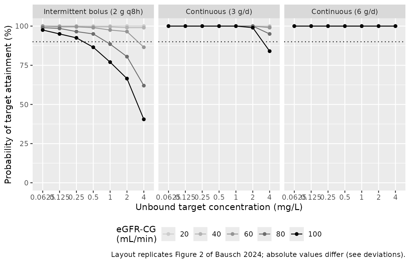
Replicates the layout of Figure 2 of Bausch 2024: probability of attaining 100% fT>target against the unbound target concentration, by eGFR-CG and regimen. See the deviations section for the quantitative discrepancy against the published panel.
# Assertions phrased as qualitative structure the model must show for ANY
# cohort it can draw, not as reproductions of the published percentages.
pta_wide <- pta |>
  tidyr::pivot_wider(names_from = regimen, values_from = pta)

# 1. Target attainment falls as renal function rises, at the clinically
#    relevant MIC-scale target, for every regimen.
at_mic <- pta |> dplyr::filter(target == 1)
stopifnot(
  all(
    at_mic |>
      dplyr::group_by(regimen) |>
      dplyr::summarise(ok = pta[CRCL == 20] >= pta[CRCL == 100], .groups = "drop") |>
      dplyr::pull(ok)
  )
)

# 2. The paper's dosing conclusion, stochastically, in the preserved-to-
#    augmented renal strata where the deterministic section showed it holds
#    (the trough ratio crosses unity near eGFR-CG 60, so this is NOT asserted
#    at 20 and 40, where intermittent dosing accumulates and wins).
stopifnot(
  all(
    pta_wide$`Continuous (3 g/d)`[pta_wide$CRCL >= 80] >=
      pta_wide$`Intermittent bolus (2 g q8h)`[pta_wide$CRCL >= 80]
  )
)

# 3. Doubling the continuous dose never lowers attainment.
stopifnot(all(pta_wide$`Continuous (6 g/d)` >= pta_wide$`Continuous (3 g/d)`))

# 4. Sanity: everything is a probability, and the easiest target/best renal
#    stratum is essentially always attained.
stopifnot(all(pta$pta >= 0), all(pta$pta <= 100))
stopifnot(
  pta |>
    dplyr::filter(target == min(pta_targets), CRCL == 20) |>
    dplyr::pull(pta) |>
    min() > 95
)
Assumptions and deviations
Monolix random effects are read as standard deviations. Table S2 reports
V_IIV0.4,Bmax_IIV0.2,CL_IOV0.4 andNS_IOV0.2 without saying whether these are variances or standard deviations. The fit was run in Monolix 2023R1 (Methods Sect. 4.7), whose population-parameter table reports random effects as the standard deviationomegaof the log-scale random effect, so the model encodes the squares (0.16, 0.04, 0.16, 0.04). The alternative reading was tested against Figure 2 and fits its head markedly worse (at eGFR-CG 100 and a 0.0625 mg/L target the SD reading gives 96% attainment against the figure’s ~96%, the variance reading 89%).Albumin acts on
NS, not onkd, against the wording of the Table S2 legend. Rationale in the Model structure section above: the Covariate Relationships block of Table S2 and the winning row of Table S3 both sayNS, and the legend gloss matches a variant the authors explicitly rejected on objective function value.Residual error is proportional only, with no additive component. Table S2 heads the residual-error block “Proportional (b)” and lists a single value for each of the total and unbound endpoints, with no additive row. Table S3 nevertheless labels the winning model’s error structure “Combined 1” (Monolix’s proportional-plus-additive form). The two are inconsistent; the model follows Table S2, because that is the table of final estimates and because no additive value is reported anywhere in the paper or supplement. Inventing one is not an option.
Four IOV occasions. The paper fits one shared IOV magnitude per parameter and never states an occasion count. Four are encoded, matching the four protocol sampling days (1, 3, 7, 14; Methods Sect. 4.4 and Figure S6), with occasions 2-4 fixed to the occasion-1 variance – the registered
$OMEGA BLOCK(1) SAME-equivalent idiom. For single-occasion data passOCC = 1.Units of
Bmaxandkd. Table S2 tabulates both without unit labels. They are encoded in mg/L, the unit of every concentration in the paper; the reproduction of the Table 2 total-concentration medians to within 1% confirms it.KNOWN DEVIATION – Figure 2 is not quantitatively reproducible from the published parameter table. The model reproduces Figure 2’s qualitative structure (attainment falls with rising renal function; continuous 3 g/d beats intermittent 6 g/d; 6 g/d continuous beats 3 g/d) but not its absolute percentages, and the gap is large. Working backwards from the published panel, the paper’s simulated steady-state trough distribution at eGFR-CG 100 on 2 g q8h is lognormal with a median near 1.1 mg/L and a log-scale SD near 1.6, whereas the packaged model’s typical trough at those covariates is 2.9 mg/L with a materially narrower spread. No reading of Table S2 – variances, standard deviations, with or without residual error, single-occasion or all-four-occasions attainment – closes that gap, and the continuous-infusion panel is inconsistent with the intermittent panel under any single clearance value. Something in the Monte Carlo setup is therefore not recoverable from what the paper prints. This is recorded as a deviation rather than gated on, and the model file’s parameters are not tuned to close it; the transcription is anchored instead on the paper’s observed Table 2 concentrations, which the model reproduces to within 1% on both total timepoints.
The continuous-vs-intermittent advantage crosses over near eGFR-CG 60 mL/min. The paper states the continuous-infusion benefit without qualifying it by renal function, but the model shows continuous 3 g/day holds a lower trough than intermittent 6 g/day below about 60 mL/min. This is a property of the published model, derived in closed form in the section above, not a transcription artefact; it is consistent with the paper’s own framing of the result as most relevant to augmented renal clearance. Assertions in this vignette are restricted accordingly.
No covariate distributions were invented. Every simulation in this vignette fixes weight, albumin and renal function at the values the paper’s own Monte Carlo used (70 kg, 24.0844 g/L, eGFR-CG 20-100 mL/min; Methods Sect. 4.7), so no assumed demographic distribution enters the validation.
No published NCA to compare against. Bausch 2024 reports concentrations and target attainment but no NCA parameters, so the PKNCA section gates on the model’s own closed-form identities rather than on a published table.