Spatial CNS and brain-tumor PBPK of abemaciclib (Wickramasinghe 2025)
Source:vignettes/articles/Wickramasinghe_2025_spatial_cns_pbpk.Rmd
Wickramasinghe_2025_spatial_cns_pbpk.RmdModel and source
ui <- rxode2::rxode(readModelDb("Wickramasinghe_2025_abemaciclib_cns_pbpk"))- Citation: Wickramasinghe CD, Kim S, Li J. SpatialCNS-PBPK: An R/Shiny Web-Based Application for Physiologically Based Pharmacokinetic Modeling of Spatial Pharmacokinetics in the Human Central Nervous System and Brain Tumors. CPT Pharmacometrics Syst Pharmacol. 2025;14(5):864-880. doi:10.1002/psp4.70026. The nine differential equations are given in Data S1 of the Supporting Information; the system-specific parameters in Table 1; the drug-specific parameter definitions in Table 2 and their abemaciclib values, the interindividual variability and the driving plasma profile in Table S2. The 9-CNS model was originally developed and validated across six drugs in Li J, Wickramasinghe C, Jiang J, et al. Clin Pharmacol Ther. 2025;117(3):690-703 (reference 7 of the 2025 tutorial), which was not available when this model was built.
- Article: https://doi.org/10.1002/psp4.70026
- PubMed Central: https://pmc.ncbi.nlm.nih.gov/articles/PMC12072228/
PBPK (9-compartment permeability-limited CNS model, SpatialCNS-PBPK R/Shiny app v1.0). Spatial pharmacokinetics of abemaciclib in the human central nervous system and brain tumors. Nine concentration states: brain blood (brain_vascular), brain parenchyma adjacent to the CSF tract (brain_csf_adjacent) and deep brain parenchyma (brain_deep), three CSF compartments (ventricular, cranial subarachnoid, spinal subarachnoid) and three tumor compartments (infiltrative rim, bulk tumor, core). Transport across the BBB, the blood-brain-tumor barrier and the blood-CSF barrier is the sum of a passive permeability-surface-area clearance acting on unbound AND unionized drug (the pH-dependent unionization fractions lam* encode the progressively acidic tumor interior) and transporter-mediated efflux and uptake clearances acting on unbound drug. CSF flows from the ventricles to the cranial and spinal subarachnoid spaces and drains to blood via arachnoid villi and nerve sheaths; drug also moves between the CSF tract and brain/tumor by paravascular (glymphatic) bulk flow and simple diffusion. The model is driven by the systemic plasma concentration supplied as the time-varying covariate CP_ABEMACICLIB_UM: plasma acts purely as a forcing function and CNS uptake does not deplete it, exactly as published. Every one of the 85 system- and drug-specific parameters is fixed to the published value; none is estimated here.
The 9-CNS model resolves the human central nervous system into nine well-stirred concentration compartments. Their canonical nlmixr2lib names and the symbols the paper uses for them are:
| nlmixr2lib state | Paper symbol | Region |
|---|---|---|
brain_vascular |
Cbb |
Brain blood (cerebral microvasculature) |
brain_csf_adjacent |
Cbm1 |
Brain parenchyma within ~2 mm of the CSF tract |
brain_deep |
Cbm2 |
Deep brain parenchyma (> 2 mm from the CSF tract) |
tumor_rim |
CT1 |
Infiltrative, non-enhancing tumor rim (pH 6.8) |
tumor_bulk |
CT2 |
Bulky, contrast-enhancing tumor (pH 6.5) |
tumor_core |
CT3 |
Tumor core (pH 6.2) |
brain_csf_ventricular |
Cvcsf |
Ventricular CSF (pH 7.3) |
brain_csf_sas_cranial |
Cccsf |
Cranial subarachnoid CSF (pH 7.3) |
brain_csf_sas_spinal |
Cscsf |
Spinal subarachnoid CSF |
Every state holds a total drug concentration.
Passive permeability moves only unbound and unionized drug, so
its driving concentration is
lam<region> * fu<region> * C<region>;
transporter-mediated clearances act on unbound drug whether ionized or
not, so theirs is fu<region> * C<region>. The
model reports both: the vignette uses the total concentrations
Cbb … Cscsf (the app’s “Total” output tabs)
and the model also returns Cbbu … Cccsfu (the
“Unbound” tabs).
Population
pop <- ui$populationThe driving plasma profile is the population-mean abemaciclib concentration-time profile determined in glioblastoma patients, attributed by this tutorial to its companion development paper (Li 2025, Clin Pharmacol Ther). Table S2 of the tutorial additionally carries paired observed abemaciclib concentrations for 39 patients who underwent tumor resection: non-enhancing tumor, contrast-enhancing tumor and CSF samples taken 120-130 h after the start of twice-daily oral dosing. No demographics (age, weight, sex, race) are reported in this paper, and the dose amount is not stated. The system-specific parameters of Table 1 describe a reference adult brain (1.2 L parenchyma, 0.15 L total CSF) carrying a 35 mL contrast-enhancing tumor.
str(pop)
#> List of 5
#>  $ species      : chr "human"
#>  $ n_subjects   : num 39
#>  $ disease_state: chr "glioblastoma (recurrent / newly diagnosed) undergoing tumor resection"
#>  $ dose_range   : chr "twice-daily oral abemaciclib; the dose amount is not stated in this paper"
#>  $ notes        : chr "The driving plasma profile in Table S2 is the population-mean abemaciclib concentration-time profile determined"| __truncated__
Source trace
Every ini() entry carries an in-file comment pointing at
its source location in
inst/modeldb/specificDrugs/Wickramasinghe_2025_abemaciclib_cns_pbpk.R.
All 85 values are fixed; none is estimated in this
paper.
| Model component | Source location |
|---|---|
| The nine differential equations | Data S1 (Supporting Information), one display equation per compartment |
Compartment volumes Vbb … Vscsf
|
Table 1 (descriptions and rounded values); Table S2 column
Sim1 (values used) |
Blood and CSF flows Qbrain, QCsink,
QSsink, QSin*, QSout*,
Qgly*
|
Table 1; Table S2 Sim1
|
Paravascular / convective bulk flows Qbulk*
|
Table 1; Table S2 Sim1
|
Passive permeability clearances PSB*,
PST*, PSV, PSC,
PSE*
|
Table 2 (definitions), Equation 1
(PSB = Papp,A-B * SA / lambda); Table S2
Sim1
|
Transporter clearances CLeff*, CLup*
|
Table 2 (definitions and the RAF scaling footnote); Table S2
Sim1
|
Brain metabolism CLmet1, CLmet2
|
Table 2; Table S2 Sim1 (both 0 for abemaciclib) |
Unbound fractions fubb … fuccsf
|
Table 2; Table S2 Sim1
|
Unionization fractions lambb …
lamccsf
|
Table 2 and its Henderson-Hasselbalch footnote; Table S2
Sim1
|
| Interindividual variability (20% CV on every parameter) | Table S2 column IIV1; lognormal form identified from
Table S3 (see Errata) |
Driving plasma profile CP_ABEMACICLIB_UM
|
Table S2 columns Time1 / Plasma1
|
| Observed tumor and CSF concentrations | Table S2 columns Ob*_T / Tumor*
|
The full per-parameter table, generated from the packaged model object:
ui$iniDf |>
  dplyr::filter(!is.na(.data$ntheta)) |>
  dplyr::transmute(
    Parameter = .data$name,
    Value = signif(ifelse(grepl("^l", .data$name), exp(.data$est), .data$est), 5),
    Scale = ifelse(grepl("^l", .data$name), "log", "linear"),
    Fixed = .data$fix,
    Description = .data$label
  ) |>
knitr::kable(caption = "All 85 fixed parameters of the 9-CNS model (Tables 1, 2 and S2).")| Parameter | Value | Scale | Fixed | Description |
|---|---|---|---|---|
| lVbb | 0.0630 | log | TRUE | Volume of brain blood (L) |
| lVbm1 | 0.1200 | log | TRUE | Volume of brain parenchyma adjacent to the CSF tract (L) |
| lVbm2 | 1.0800 | log | TRUE | Volume of deep brain parenchyma (L) |
| lVT1 | 0.0700 | log | TRUE | Volume of the infiltrative tumor rim (L) |
| lVT2 | 0.0350 | log | TRUE | Volume of the bulky tumor region (L) |
| lVT3 | 0.0035 | log | TRUE | Volume of the tumor core (L) |
| lVvcsf | 0.0250 | log | TRUE | Volume of ventricular CSF (L) |
| lVccsf | 0.0450 | log | TRUE | Volume of cranial subarachnoid CSF (L) |
| lVscsf | 0.0800 | log | TRUE | Volume of spinal subarachnoid CSF (L) |
| lQbrain | 39.0000 | log | TRUE | Cerebral blood flow (L/h) |
| lQCsink | 0.0130 | log | TRUE | Absorption rate of cranial CSF into blood via arachnoid villi (L/h) |
| lQSsink | 0.0080 | log | TRUE | Absorption rate of spinal CSF into blood via arachnoid villi (L/h) |
| lQbulkCB1 | 0.0013 | log | TRUE | Paravascular bulk flow rate, cranial subarachnoid CSF to brain parenchyma 1 (L/h) |
| lQbulkB1C | 0.0016 | log | TRUE | Paravascular bulk flow rate, brain parenchyma 1 to cranial subarachnoid CSF (L/h) |
| lQbulkVB1 | 0.0001 | log | TRUE | Paravascular bulk flow rate, ventricular CSF to brain parenchyma 1 (L/h) |
| lQbulkB1V | 0.0002 | log | TRUE | Paravascular bulk flow rate, brain parenchyma 1 to ventricular CSF (L/h) |
| lQbulkB2B1 | 0.0005 | log | TRUE | Convective bulk flow rate, brain parenchyma 2 to 1 (L/h) |
| lQbulkB1B2 | 0.0005 | log | TRUE | Convective bulk flow rate, brain parenchyma 1 to 2 (L/h) |
| lQbulkB2T1 | 0.0005 | log | TRUE | Convective bulk flow rate, brain parenchyma 2 to tumor rim (L/h) |
| lQbulkT1B2 | 0.0005 | log | TRUE | Convective bulk flow rate, tumor rim to brain parenchyma 2 (L/h) |
| lQbulkCB2 | 0.0113 | log | TRUE | Paravascular bulk flow rate, cranial subarachnoid CSF to brain parenchyma 2 (L/h) |
| lQbulkB2C | 0.0142 | log | TRUE | Paravascular bulk flow rate, brain parenchyma 2 to cranial subarachnoid CSF (L/h) |
| lQbulkT2T1 | 0.0002 | log | TRUE | Convective bulk flow rate, bulk tumor to tumor rim (L/h) |
| lQbulkT1T2 | 0.0002 | log | TRUE | Convective bulk flow rate, tumor rim to bulk tumor (L/h) |
| lQbulkCT1 | 0.0013 | log | TRUE | Paravascular bulk flow rate, cranial subarachnoid CSF to tumor rim (L/h) |
| lQbulkT1C | 0.0016 | log | TRUE | Paravascular bulk flow rate, tumor rim to cranial subarachnoid CSF (L/h) |
| lQbulkT3T2 | 0.0002 | log | TRUE | Convective bulk flow rate, tumor core to bulk tumor (L/h) |
| lQbulkT2T3 | 0.0002 | log | TRUE | Convective bulk flow rate, bulk tumor to tumor core (L/h) |
| lQbulkCT2 | 0.0002 | log | TRUE | Paravascular bulk flow rate, cranial subarachnoid CSF to bulk tumor (L/h) |
| lQbulkT2C | 0.0003 | log | TRUE | Paravascular bulk flow rate, bulk tumor to cranial subarachnoid CSF (L/h) |
| lQbulkCT3 | 0.0002 | log | TRUE | Paravascular bulk flow rate, cranial subarachnoid CSF to tumor core (L/h) |
| lQbulkT3C | 0.0002 | log | TRUE | Paravascular bulk flow rate, tumor core to cranial subarachnoid CSF (L/h) |
| lQSin1r | 0.0013 | log | TRUE | CSF back-flow rate from the cranial subarachnoid space to the ventricle (L/h) |
| lQSin1 | 0.0126 | log | TRUE | CSF flow rate from the ventricle to the cranial subarachnoid space (L/h) |
| lQSin2r | 0.0008 | log | TRUE | CSF back-flow rate from the spinal subarachnoid space to the ventricle (L/h) |
| lQSin2 | 0.0084 | log | TRUE | CSF flow rate from the ventricle to the spinal subarachnoid space (L/h) |
| lQSout | 0.0004 | log | TRUE | CSF flow rate from the spinal to the cranial subarachnoid space (L/h) |
| QSoutr | 0.0000 | linear | TRUE | CSF flow rate from the cranial to the spinal subarachnoid space (L/h) |
| lPSB1 | 2.5480 | log | TRUE | Passive permeability clearance at the BBB, brain blood to adjacent brain parenchyma (L/h) |
| lPSB2 | 25.4800 | log | TRUE | Passive permeability clearance at the BBB, brain blood to deep brain parenchyma (L/h) |
| lPST1 | 2.0384 | log | TRUE | Passive permeability clearance at the BBTB, brain blood to tumor rim (L/h) |
| lPST2 | 5.0960 | log | TRUE | Passive permeability clearance at the BBTB, brain blood to bulk tumor (L/h) |
| lPST3 | 0.5096 | log | TRUE | Passive permeability clearance at the BBTB, brain blood to tumor core (L/h) |
| lPSV | 0.8408 | log | TRUE | Passive permeability clearance at the blood-CSF barrier, brain blood to ventricular CSF (L/h) |
| lPSC | 1.7072 | log | TRUE | Passive permeability clearance at the blood-CSF barrier, brain blood to cranial subarachnoid CSF (L/h) |
| lPSE1 | 50.9600 | log | TRUE | Simple diffusion rate between cranial subarachnoid CSF and adjacent brain parenchyma (L/h) |
| lPSE2 | 25.4800 | log | TRUE | Simple diffusion rate between ventricular CSF and adjacent brain parenchyma (L/h) |
| lPSB1B2 | 0.0100 | log | TRUE | Simple diffusion rate between the adjacent and deep brain parenchyma (L/h) |
| lPSB2T1 | 0.0100 | log | TRUE | Simple diffusion rate between the deep brain parenchyma and tumor rim (L/h) |
| lPST1T2 | 0.0100 | log | TRUE | Simple diffusion rate between tumor rim and bulk tumor (L/h) |
| lPST2T3 | 0.0100 | log | TRUE | Simple diffusion rate between bulk tumor and tumor core (L/h) |
| lCLeffbbb1 | 0.2920 | log | TRUE | Efflux transporter-mediated clearance at the BBB, brain blood to adjacent brain parenchyma (L/h) |
| CLupbbb1 | 0.0000 | linear | TRUE | Uptake transporter-mediated influx clearance at the BBB, brain blood to adjacent brain parenchyma (L/h) |
| lCLeffbbb2 | 2.9200 | log | TRUE | Efflux transporter-mediated clearance at the BBB, brain blood to deep brain parenchyma (L/h) |
| CLupbbb2 | 0.0000 | linear | TRUE | Uptake transporter-mediated influx clearance at the BBB, brain blood to deep brain parenchyma (L/h) |
| lCLeffT1 | 0.0584 | log | TRUE | Efflux transporter-mediated clearance at the BBTB, brain blood to tumor rim (L/h) |
| CLupT1 | 0.0000 | linear | TRUE | Uptake transporter-mediated influx clearance at the BBB, brain blood to tumor rim (L/h) |
| lCLeffT2 | 0.0088 | log | TRUE | Efflux transporter-mediated clearance at the BBTB, brain blood to bulk tumor (L/h) |
| CLupT2 | 0.0000 | linear | TRUE | Uptake transporter-mediated influx clearance at the BBB, brain blood to bulk tumor (L/h) |
| CLeffT3 | 0.0000 | linear | TRUE | Efflux transporter-mediated clearance at the BBTB, brain blood to tumor core (L/h) |
| CLupT3 | 0.0000 | linear | TRUE | Uptake transporter-mediated influx clearance at the BBB, brain blood to tumor core (L/h) |
| CLeffvcsf | 0.0000 | linear | TRUE | Efflux transporter-mediated clearance at the blood-CSF barrier, brain blood to ventricular CSF (L/h) |
| CLupvcsf | 0.0000 | linear | TRUE | Uptake transporter-mediated clearance at the blood-CSF barrier, brain blood to ventricular CSF (L/h) |
| CLeffccsf | 0.0000 | linear | TRUE | Efflux transporter-mediated clearance at the blood-CSF barrier, brain blood to cranial subarachnoid CSF (L/h) |
| CLupccsf | 0.0000 | linear | TRUE | Uptake transporter-mediated clearance at the blood-CSF barrier, brain blood to cranial subarachnoid CSF (L/h) |
| CLmet1 | 0.0000 | linear | TRUE | Drug metabolism clearance in the adjacent brain parenchyma (L/h) |
| CLmet2 | 0.0000 | linear | TRUE | Drug metabolism clearance in the deep brain parenchyma (L/h) |
| lfubb | 0.0260 | log | TRUE | Unbound fraction in brain blood (fraction) |
| lfubm1 | 0.0060 | log | TRUE | Unbound fraction in the adjacent brain parenchyma (fraction) |
| lfubm2 | 0.0060 | log | TRUE | Unbound fraction in the deep brain parenchyma (fraction) |
| lfuT1 | 0.0090 | log | TRUE | Unbound fraction in the tumor rim (fraction) |
| lfuT2 | 0.0160 | log | TRUE | Unbound fraction in the bulk tumor (fraction) |
| lfuT3 | 0.0160 | log | TRUE | Unbound fraction in the tumor core (fraction) |
| lfuvcsf | 0.2890 | log | TRUE | Unbound fraction in ventricular CSF (fraction) |
| lfuccsf | 0.2890 | log | TRUE | Unbound fraction in cranial subarachnoid CSF (fraction) |
| llambb | 0.2238 | log | TRUE | Unionization fraction in brain blood (pH 7.4) (fraction) |
| llambm1 | 0.1540 | log | TRUE | Unionization fraction in the adjacent brain parenchyma (pH 7.2) (fraction) |
| llambm2 | 0.1540 | log | TRUE | Unionization fraction in the deep brain parenchyma (pH 7.2) (fraction) |
| llamT1 | 0.0676 | log | TRUE | Unionization fraction in the tumor rim (pH 6.8) (fraction) |
| llamT2 | 0.0350 | log | TRUE | Unionization fraction in the bulk tumor (pH 6.5) (fraction) |
| llamT3 | 0.0114 | log | TRUE | Unionization fraction in the tumor core (pH 6.2) (fraction) |
| llamvcsf | 0.1864 | log | TRUE | Unionization fraction in ventricular CSF (pH 7.3) (fraction) |
| llamccsf | 0.1864 | log | TRUE | Unionization fraction in cranial subarachnoid CSF (pH 7.3) (fraction) |
| lQglyccsf | 0.0065 | log | TRUE | Absorption rate of cranial CSF via olfactory mucosa and cranial nerve sheaths (L/h) |
| lQglyscsf | 0.0040 | log | TRUE | Absorption rate of spinal CSF via spinal nerve sheaths (L/h) |
The input function
The 9-CNS model is driven by the systemic plasma concentration
supplied as the time-varying covariate CP_ABEMACICLIB_UM.
Plasma is a pure forcing function: CNS uptake never depletes it, so the
coupling is one-way. The 1010-point population-mean profile of Table S2
is shipped with the package.
plasma <- read.csv(
  system.file("extdata", "Wickramasinghe_2025_abemaciclib_plasma_input.csv",
              package = "nlmixr2lib")
)
observed <- read.csv(
  system.file("extdata", "Wickramasinghe_2025_abemaciclib_observed_cns.csv",
              package = "nlmixr2lib")
)
stopifnot(nrow(plasma) == 1010L, nrow(observed) == 110L)

c(n_points = nrow(plasma),
  t_max = max(plasma$time),
  Cmax = max(plasma$CP_ABEMACICLIB_UM),
  t_at_Cmax = plasma$time[which.max(plasma$CP_ABEMACICLIB_UM)])
#>  n_points     t_max      Cmax t_at_Cmax
#> 1010.0000  168.0000    0.4191  124.6100
ggplot(plasma, aes(time, CP_ABEMACICLIB_UM)) +
  geom_line() +
  scale_y_log10() +
  labs(x = "Time (h)", y = "Plasma abemaciclib (umol/L)",
       title = "Input function: population-mean plasma profile",
       caption = "Table S2 columns Time1 / Plasma1 of Wickramasinghe 2025.")
#> Warning in scale_y_log10(): log-10 transformation introduced infinite values.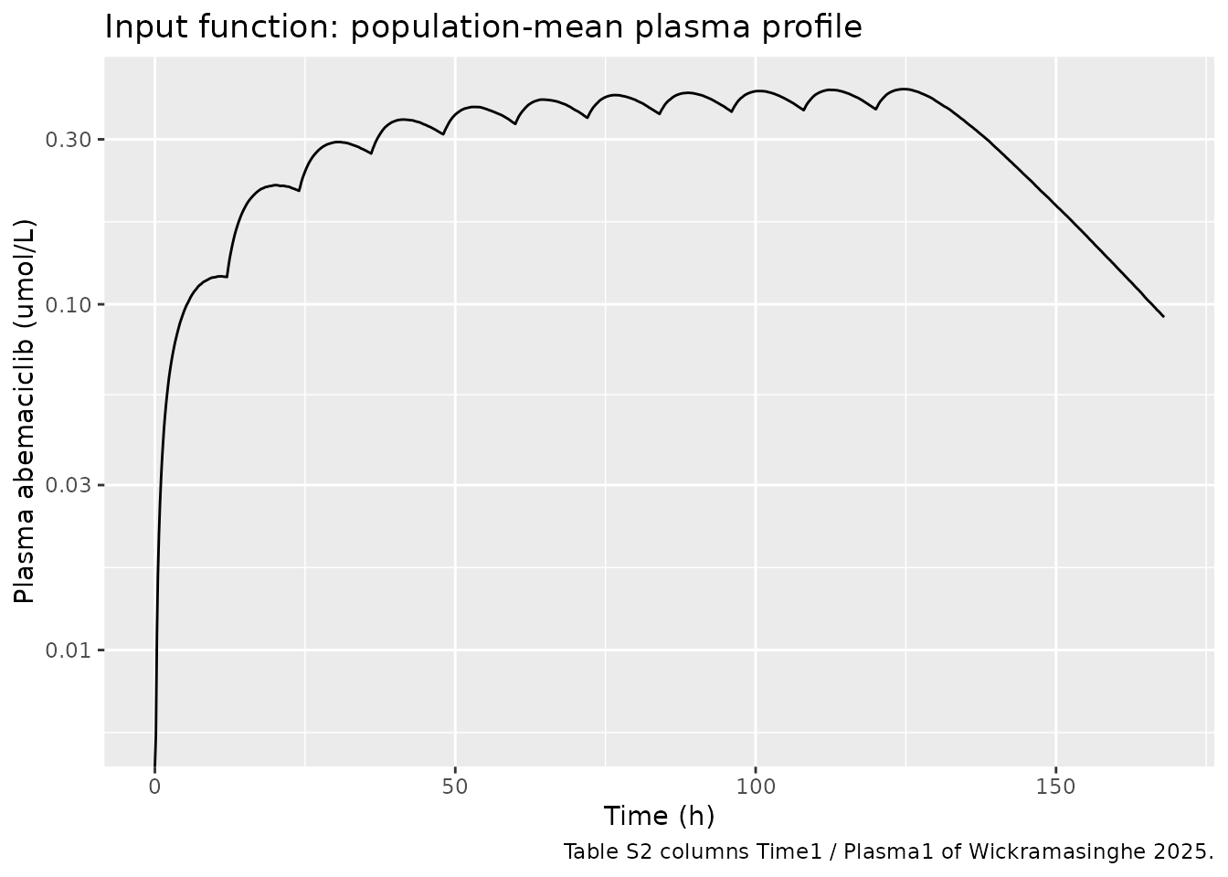
The covariate must be interpolated linearly, as the app does. The output grid of every simulation below is therefore the published 1010-point grid itself: coarsening it to 0.7 h changes the predicted CNS concentrations by up to 3%, so the profile is used at full resolution rather than thinned.
Typical-value simulation: replicating Figure 2
Figure 2 of the paper is a screenshot of the app’s “Concentration log plots (Total)” tab: the mean total-concentration profile in each compartment, with the observed tumor and CSF concentrations overlaid. It is a typical-value prediction, so the random effects are zeroed.
mod_typical <- rxode2::zeroRe(readModelDb("Wickramasinghe_2025_abemaciclib_cns_pbpk"))
#> Warning: No sigma parameters in the model

events_typical <- data.frame(
  id = 1L,
  time = plasma$time,
  amt = NA_real_,
  evid = 0L,
  cmt = "brain_vascular",
  CP_ABEMACICLIB_UM = plasma$CP_ABEMACICLIB_UM
)

sim_typical <- rxode2::rxSolve(
  mod_typical, events_typical,
  covsInterpolation = "linear", returnType = "data.frame"
)
#> ℹ omega/sigma items treated as zero: 'etalVbb', 'etalVbm1', 'etalVbm2', 'etalVT1', 'etalVT2', 'etalVT3', 'etalVvcsf', 'etalVccsf', 'etalVscsf', 'etalQbrain', 'etalQCsink', 'etalQSsink', 'etalQbulkCB1', 'etalQbulkB1C', 'etalQbulkVB1', 'etalQbulkB1V', 'etalQbulkB2B1', 'etalQbulkB1B2', 'etalQbulkB2T1', 'etalQbulkT1B2', 'etalQbulkCB2', 'etalQbulkB2C', 'etalQbulkT2T1', 'etalQbulkT1T2', 'etalQbulkCT1', 'etalQbulkT1C', 'etalQbulkT3T2', 'etalQbulkT2T3', 'etalQbulkCT2', 'etalQbulkT2C', 'etalQbulkCT3', 'etalQbulkT3C', 'etalQSin1r', 'etalQSin1', 'etalQSin2r', 'etalQSin2', 'etalQSout', 'etalPSB1', 'etalPSB2', 'etalPST1', 'etalPST2', 'etalPST3', 'etalPSV', 'etalPSC', 'etalPSE1', 'etalPSE2', 'etalPSB1B2', 'etalPSB2T1', 'etalPST1T2', 'etalPST2T3', 'etalCLeffbbb1', 'etalCLeffbbb2', 'etalCLeffT1', 'etalCLeffT2', 'etalfubb', 'etalfubm1', 'etalfubm2', 'etalfuT1', 'etalfuT2', 'etalfuT3', 'etalfuvcsf', 'etalfuccsf', 'etallambb', 'etallambm1', 'etallambm2', 'etallamT1', 'etallamT2', 'etallamT3', 'etallamvcsf', 'etallamccsf', 'etalQglyccsf', 'etalQglyscsf'
if (is.null(sim_typical$id)) sim_typical$id <- 1L
nrow(sim_typical)
#> [1] 1010
# Replicates Figure 2 of Wickramasinghe 2025: mean total abemaciclib
# concentration-time profile in each of the nine CNS compartments, on a
# log10 axis, with the observed tumor and CSF concentrations overlaid.
panel_levels <- c(
  Cbb = "Cbb (brain blood)",
  Cbm1 = "Cbm1 (parenchyma adj. CSF)",
  Cbm2 = "Cbm2 (deep parenchyma)",
  CT1 = "CT1 (tumor rim)",
  CT2 = "CT2 (bulk tumor)",
  CT3 = "CT3 (tumor core)",
  Cvcsf = "Cvcsf (ventricular CSF)",
  Cccsf = "Cccsf (cranial SAS CSF)",
  Cscsf = "Cscsf (spinal SAS CSF)"
)

pred_long <- sim_typical |>
  dplyr::select(time, dplyr::all_of(names(panel_levels))) |>
  tidyr::pivot_longer(-time, names_to = "state", values_to = "conc") |>
  dplyr::mutate(panel = factor(panel_levels[state], levels = panel_levels))

# The paper overlays the tumor observations on Cbm2/CT1/CT2/CT3 and the CSF
# observations on Cvcsf/Cccsf/Cscsf (Figure 2 caption).
obs_long <- dplyr::bind_rows(
  observed |> dplyr::filter(matrix != "CSF") |>
    tidyr::crossing(state = c("Cbm2", "CT1", "CT2", "CT3")),
  observed |> dplyr::filter(matrix == "CSF") |>
    tidyr::crossing(state = c("Cvcsf", "Cccsf", "Cscsf"))
) |>
  dplyr::mutate(panel = factor(panel_levels[state], levels = panel_levels))

ggplot(pred_long, aes(time, conc)) +
  geom_line(colour = "blue") +
  geom_point(data = obs_long, aes(time, conc, colour = matrix, shape = matrix),
             alpha = 0.7, size = 1.3) +
  facet_wrap(~panel, ncol = 2, scales = "free_y") +
  scale_y_log10() +
  scale_colour_manual(values = c("CSF" = "darkgreen",
                                 "enhancing tumor" = "red",
                                 "non-enhancing tumor" = "black")) +
  labs(x = "Time (h)", y = "Total abemaciclib (umol/L)", colour = NULL, shape = NULL,
       title = "Figure 2 - simulated mean total concentration by CNS compartment",
       caption = "Replicates Figure 2 of Wickramasinghe 2025.") +
  theme(legend.position = "bottom")
#> Warning in scale_y_log10(): log-10 transformation introduced infinite values.
#> log-10 transformation introduced infinite values.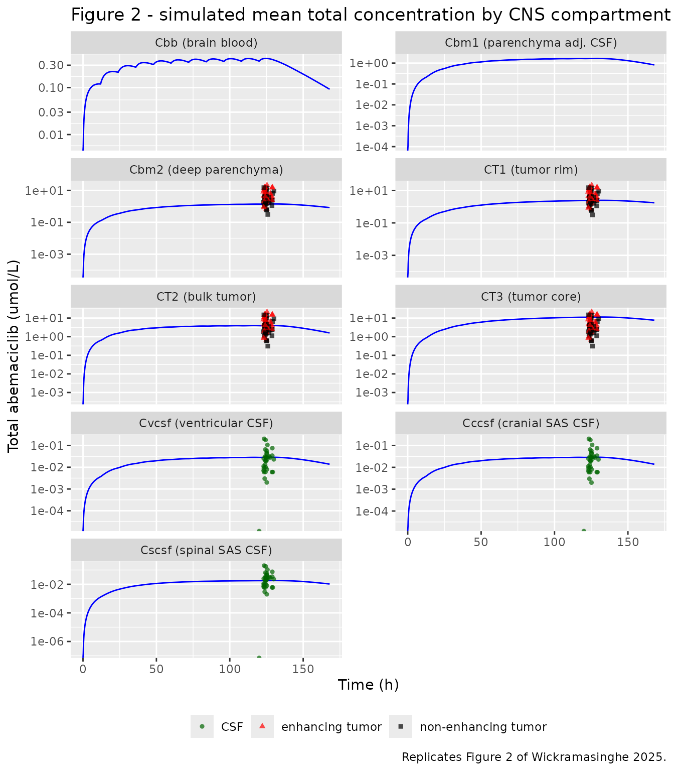
Quantitative check against Figure 2
Figure 2 is a log10-axis screenshot, so it can only be read to about a half-decade. The check below pins each panel’s value at the steady-state peak (t = 124.61 h, the time of the plasma Cmax) against the value read off the published figure.
t_peak <- plasma$time[which.max(plasma$CP_ABEMACICLIB_UM)]
i_peak <- which.min(abs(sim_typical$time - t_peak))

fig2_read <- c(Cbb = 0.42, Cbm1 = 1.6, Cbm2 = 1.5, CT1 = 2.5, CT2 = 4,
               CT3 = 11, Cvcsf = 0.03, Cccsf = 0.03, Cscsf = NA)

fig2_cmp <- tibble::tibble(
  Compartment = names(panel_levels),
  Simulated = signif(unlist(sim_typical[i_peak, names(panel_levels)]), 4),
  `Read off Figure 2` = unname(fig2_read[names(panel_levels)])
) |>
  dplyr::mutate(`Ratio` = signif(Simulated / `Read off Figure 2`, 3))

knitr::kable(
  fig2_cmp,
  caption = paste0("Total concentration at the steady-state plasma peak (t = ",
                   round(t_peak, 2), " h). Cscsf is not shown in Figure 2.")
)| Compartment | Simulated | Read off Figure 2 | Ratio |
|---|---|---|---|
| Cbb | 0.41890 | 0.42 | 0.997 |
| Cbm1 | 1.65900 | 1.60 | 1.040 |
| Cbm2 | 1.39400 | 1.50 | 0.929 |
| CT1 | 2.42900 | 2.50 | 0.972 |
| CT2 | 3.94000 | 4.00 | 0.985 |
| CT3 | 11.21000 | 11.00 | 1.020 |
| Cvcsf | 0.02860 | 0.03 | 0.953 |
| Cccsf | 0.02885 | 0.03 | 0.962 |
| Cscsf | 0.01802 | NA | NA |
# A log10 screenshot can only be read to about a half-decade, but the model
# agrees with every readable panel far more tightly than that (worst case
# 0.033 in log10, i.e. 8%). Assert the accuracy actually achieved, so this is
# a regression guard rather than a formality.
ok <- !is.na(fig2_cmp$`Read off Figure 2`)
stopifnot(sum(ok) == 8L, all(abs(log10(fig2_cmp$Ratio[ok])) < 0.05))
The brain-blood compartment equilibrates with plasma almost instantly
(Qbrain = 39 L/h into Vbb = 0.063 L), so
Cbb tracks the input function exactly. That is the model
behaving as published, not a degenerate case:
The spatial gradient the model exists to predict
The whole point of resolving nine compartments rather than one is that the predicted exposure is not uniform across the CNS. At the steady-state peak the model predicts a monotone rise from CSF through parenchyma into the progressively more disrupted tumor interior:
gradient <- sim_typical[i_peak, c("Cccsf", "Cbm2", "CT1", "CT2", "CT3")]
stopifnot(all(diff(unlist(gradient)) > 0))
tibble::tibble(
  Region = c("Cranial SAS CSF", "Deep parenchyma", "Tumor rim",
             "Bulk tumor", "Tumor core"),
  `Total (umol/L)` = signif(unlist(gradient), 3),
  `Fold vs CSF` = signif(unlist(gradient) / gradient$Cccsf, 3)
) |>
knitr::kable(caption = "Predicted spatial gradient at the steady-state peak.")| Region | Total (umol/L) | Fold vs CSF |
|---|---|---|
| Cranial SAS CSF | 0.0289 | 1.0 |
| Deep parenchyma | 1.3900 | 48.3 |
| Tumor rim | 2.4300 | 84.2 |
| Bulk tumor | 3.9400 | 137.0 |
| Tumor core | 11.2000 | 389.0 |
Comparison against the observed patient data
The observed concentrations in Table S2 are the paper’s own
validation data. The model prediction is compared at each patient’s
actual sampling time, using the compartment the paper pairs with each
matrix: the non-enhancing tumor with tumor_rim
(CT1), the contrast-enhancing tumor with
tumor_bulk (CT2) and CSF with
brain_csf_sas_cranial (Cccsf).
state_for <- c("non-enhancing tumor" = "CT1",
               "enhancing tumor" = "CT2",
               "CSF" = "Cccsf")

pred_at <- function(state, times) {
  stats::approx(sim_typical$time, sim_typical[[state]], xout = times, rule = 2)$y
}

obs_cmp <- observed |>
  dplyr::mutate(
    state = unname(state_for[matrix]),
    predicted = mapply(pred_at, state, time),
    ratio = conc / predicted
  )
stopifnot(nrow(obs_cmp) == 110L, !anyNA(obs_cmp$predicted))

obs_cmp |>
  dplyr::group_by(Matrix = matrix) |>
  dplyr::summarise(
    N = dplyr::n(),
    `Paired compartment` = dplyr::first(state),
    `Observed median` = signif(stats::median(conc), 3),
    `Predicted (typical)` = signif(stats::median(predicted), 3),
    `Median obs/pred` = signif(stats::median(ratio), 3),
    `5th-95th pct of obs/pred` = paste(
      signif(stats::quantile(ratio, 0.05), 2), "-",
      signif(stats::quantile(ratio, 0.95), 2)
    ),
    .groups = "drop"
  ) |>
  knitr::kable(caption = paste(
    "Observed abemaciclib concentrations (Table S2, 39 glioblastoma patients)",
    "against the typical-value prediction at each patient's sampling time."
))| Matrix | N | Paired compartment | Observed median | Predicted (typical) | Median obs/pred | 5th-95th pct of obs/pred |
|---|---|---|---|---|---|---|
| CSF | 34 | Cccsf | 0.024 | 0.0289 | 0.833 | 0.092 - 4.6 |
| enhancing tumor | 37 | CT2 | 4.440 | 3.9400 | 1.130 | 0.25 - 4 |
| non-enhancing tumor | 39 | CT1 | 2.600 | 2.4300 | 1.070 | 0.25 - 5.8 |
The typical-value prediction sits inside the observed spread for all three matrices, which is the claim Figure 2 makes graphically. The observed between-patient spread is far wider than the template’s uniform 20% CV produces (see Errata) - the paper does not fit that spread, and neither does this vignette.
med_ratio <- obs_cmp |>
  dplyr::group_by(matrix) |>
  dplyr::summarise(m = stats::median(ratio), .groups = "drop")
# The typical-value prediction must land within 3-fold of the observed median
# in every matrix -- a real constraint given the predictions span 0.03 to 11
# umol/L across compartments.
stopifnot(nrow(med_ratio) == 3L, all(med_ratio$m > 1 / 3), all(med_ratio$m < 3))
signif(stats::setNames(med_ratio$m, med_ratio$matrix), 3)
#>                 CSF     enhancing tumor non-enhancing tumor
#>               0.833               1.130               1.070
Virtual cohort with interindividual variability
Table S2 assigns the same 20% CV to every one of the 85 parameters and the app uses it to generate individual profiles (its “individual concentration - time profiles” tab). The cohort below is 100 virtual patients - well inside the 200-per-arm cap and matching the scale of the app’s own default group size.
set.seed(20250518)
n_sub <- 100L

events_cohort <- data.frame(
  id = rep(seq_len(n_sub), each = nrow(plasma)),
  time = rep(plasma$time, times = n_sub),
  amt = NA_real_,
  evid = 0L,
  cmt = "brain_vascular",
  CP_ABEMACICLIB_UM = rep(plasma$CP_ABEMACICLIB_UM, times = n_sub)
)
stopifnot(!anyDuplicated(events_cohort[, c("id", "time", "evid")]))

sim_cohort <- rxode2::rxSolve(
  readModelDb("Wickramasinghe_2025_abemaciclib_cns_pbpk"),
  events_cohort,
  covsInterpolation = "linear", returnType = "data.frame"
)
dplyr::n_distinct(sim_cohort$id)
#> [1] 100
The IIV reproduces the app’s own virtual patients
Table S3 lists five virtual patients that the SpatialCNS-PBPK app
generated from Sim1 + IIV1. Those draws
identify the distributional form the paper never states: across the 355
non-zero parameter draws, log(simulated / typical) is
normal (Shapiro-Wilk p = 0.15, skewness 0.12) with SD 0.194 against the
sqrt(log(1 + 0.20^2)) = 0.198 expected of a 20% CV
lognormal, while the untransformed ratios are clearly right-skewed
(Shapiro-Wilk p = 1.6e-8, skewness 0.94). The packaged model encodes
that lognormal form; the check below confirms the simulated cohort
returns the 20% CV.
sim_par <- sim_cohort |>
  dplyr::distinct(id, .keep_all = TRUE) |>
  dplyr::select(PSB2, CLeffbbb2, fubb, VT2, lamT1)

cv <- vapply(sim_par, function(x) stats::sd(x) / mean(x), numeric(1))
tibble::tibble(
  Parameter = names(cv),
  `Simulated CV` = signif(cv, 3),
  `Table S2 IIV1` = 0.20
) |>
knitr::kable(caption = "Realised interindividual CV in the 100-patient cohort.")| Parameter | Simulated CV | Table S2 IIV1 |
|---|---|---|
| PSB2 | 0.193 | 0.2 |
| CLeffbbb2 | 0.218 | 0.2 |
| fubb | 0.206 | 0.2 |
| VT2 | 0.195 | 0.2 |
| lamT1 | 0.221 | 0.2 |
Variability bands by compartment
sim_cohort |>
  dplyr::select(id, time, dplyr::all_of(names(panel_levels))) |>
  tidyr::pivot_longer(-c(id, time), names_to = "state", values_to = "conc") |>
  dplyr::group_by(state, time) |>
  dplyr::summarise(
    Q05 = stats::quantile(conc, 0.05),
    Q50 = stats::quantile(conc, 0.50),
    Q95 = stats::quantile(conc, 0.95),
    .groups = "drop"
  ) |>
  dplyr::mutate(panel = factor(panel_levels[state], levels = panel_levels)) |>
  ggplot(aes(time, Q50)) +
  geom_ribbon(aes(ymin = Q05, ymax = Q95), alpha = 0.25, fill = "steelblue") +
  geom_line(colour = "steelblue4") +
  facet_wrap(~panel, ncol = 2, scales = "free_y") +
  scale_y_log10() +
  labs(x = "Time (h)", y = "Total abemaciclib (umol/L)",
       title = "Median and 5th-95th percentile profiles, 100 virtual patients",
       caption = paste("Reproduces the app's mean-and-individual-profiles output",
                       "using the Table S2 IIV1 column."))
#> Warning in scale_y_log10(): log-10 transformation introduced infinite values.
#> log-10 transformation introduced infinite values.
#> log-10 transformation introduced infinite values.
#> log-10 transformation introduced infinite values.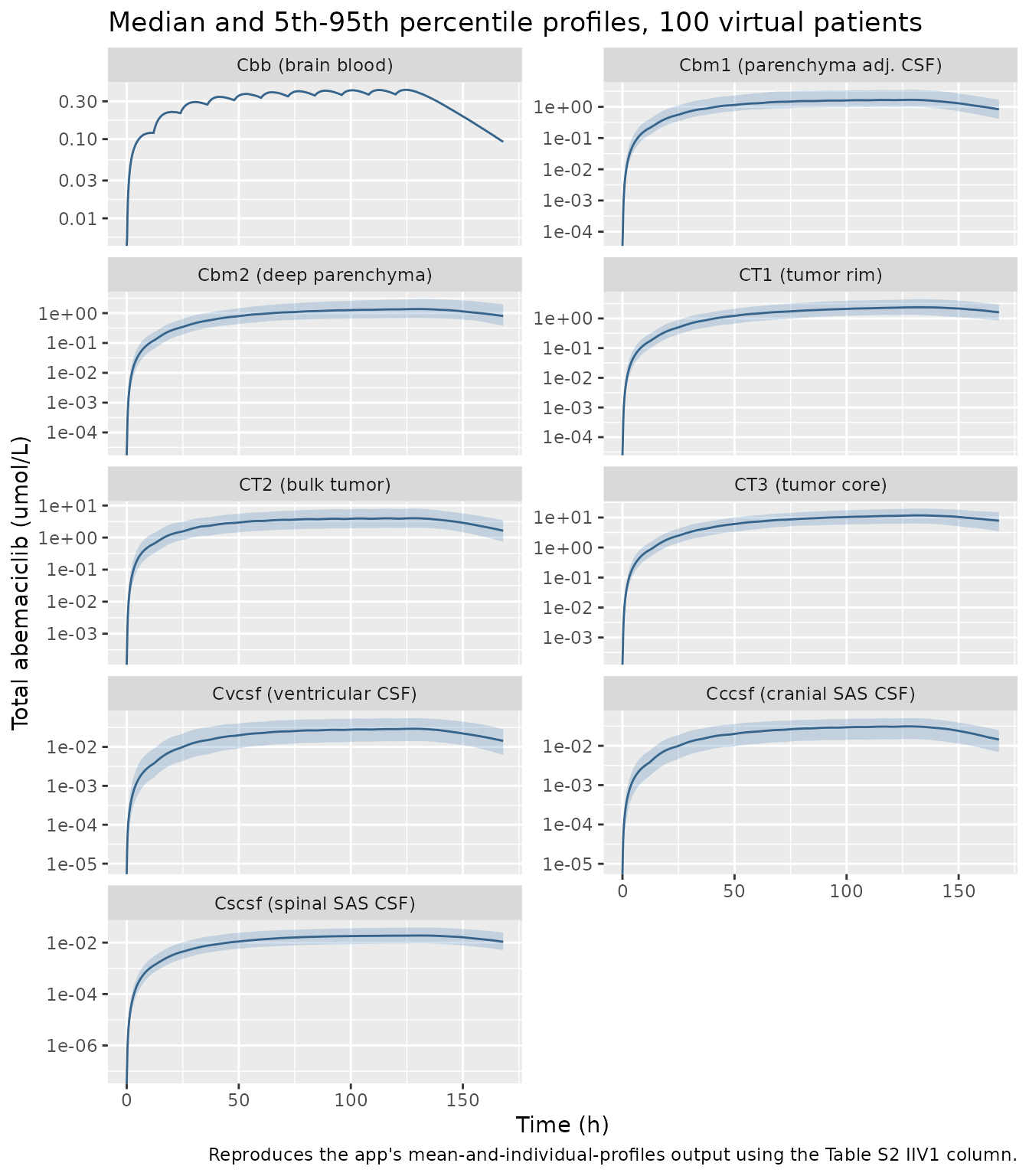
PKNCA validation
The app computes Cmax, Tmax and AUC over a user-selected window; the paper’s own worked example is “any user-defined time interval (e.g., 72-96 h)”. The same window is used here, one NCA per compartment. Note that 72-96 h is a 24 h dosing day part-way through the accumulation phase, not a steady-state interval: the plasma peaks are still climbing at that point (0.391 umol/L at 64 h against 0.419 umol/L at 124.6 h), and the CNS compartments are further from equilibrium still.
nca_states <- names(panel_levels)

sim_nca <- sim_cohort |>
  dplyr::select(id, time, dplyr::all_of(nca_states)) |>
  tidyr::pivot_longer(-c(id, time), names_to = "compartment", values_to = "Cc") |>
  dplyr::filter(!is.na(Cc))

# Guarantee a time = 0 record per (id, compartment). Every CNS compartment
# starts empty, so Cc = 0 at t = 0 is the correct anchor.
sim_nca <- dplyr::bind_rows(
  sim_nca,
  sim_nca |> dplyr::distinct(id, compartment) |>
    dplyr::mutate(time = 0, Cc = 0)
) |>
  dplyr::distinct(id, compartment, time, .keep_all = TRUE) |>
  dplyr::arrange(compartment, id, time)

stopifnot(nrow(sim_nca) > 0, all(sim_nca$Cc >= 0))

conc_obj <- PKNCA::PKNCAconc(sim_nca, Cc ~ time | compartment + id)

intervals <- data.frame(
  start = 72, end = 96,
  cmax = TRUE, tmax = TRUE, cmin = TRUE, auclast = TRUE
)

# There are no dose events in this model -- the systemic PK enters as a
# covariate -- so the NCA runs without a PKNCAdose object.
nca_res <- PKNCA::pk.nca(
  PKNCA::PKNCAdata(conc_obj, data.dose = NA, intervals = intervals)
)
#> No dose information provided, calculations requiring dose will return NA.
nca_tab <- as.data.frame(nca_res) |>
  dplyr::group_by(compartment, PPTESTCD) |>
  dplyr::summarise(value = stats::median(PPORRES), .groups = "drop") |>
  tidyr::pivot_wider(names_from = PPTESTCD, values_from = value) |>
  dplyr::mutate(
    compartment = factor(compartment, levels = nca_states),
    dplyr::across(dplyr::where(is.numeric), ~ signif(.x, 3))
  ) |>
  dplyr::arrange(compartment)

nca_tab |>
  dplyr::rename(
    "Compartment" = compartment,
    "Cmax (umol/L)" = cmax,
    "Cmin (umol/L)" = cmin,
    "Tmax (h)" = tmax,
    "AUC72-96 (umol*h/L)" = auclast
  ) |>
  knitr::kable(caption = paste(
    "Median NCA parameters over the app's default 72-96 h window,",
    "100 virtual patients."
))| Compartment | AUC72-96 (umol*h/L) | Cmax (umol/L) | Cmin (umol/L) | Tmax (h) |
|---|---|---|---|---|
| Cbb | 9.310 | 0.4090 | 0.3460 | 16.8 |
| Cbm1 | 36.700 | 1.5900 | 1.4500 | 22.3 |
| Cbm2 | 28.000 | 1.2500 | 1.0700 | 24.0 |
| CT1 | 45.300 | 2.0500 | 1.6800 | 24.0 |
| CT2 | 90.300 | 3.8800 | 3.5700 | 21.2 |
| CT3 | 224.000 | 10.2000 | 8.4100 | 24.0 |
| Cvcsf | 0.639 | 0.0275 | 0.0250 | 21.3 |
| Cccsf | 0.666 | 0.0291 | 0.0256 | 21.7 |
| Cscsf | 0.404 | 0.0178 | 0.0155 | 24.0 |
No published NCA table to compare against. This
tutorial demonstrates the app’s pharmacokinetic-parameter function but
does not print numeric Cmax / Tmax / AUC values for abemaciclib anywhere
in the paper or its supplement, so there is no reference row for
ncaComparisonTable(). The table above is therefore a
functional check of the packaged model rather than a comparison against
published values; the quantitative validation of this extraction rests
on the Figure 2 replication and the observed-data comparison above.
The NCA does support two internal consistency checks:
# 1. Peak-to-trough ordering must hold in every compartment.
stopifnot(all(nca_tab$cmax >= nca_tab$cmin))

# 2. Over a 24 h window, AUC72-96 must lie between 24 * Cmin and 24 * Cmax
#    for every compartment.
stopifnot(
  all(nca_tab$auclast >= 24 * nca_tab$cmin),
  all(nca_tab$auclast <= 24 * nca_tab$cmax)
)

# 3. Exposure, not just instantaneous concentration, must rise monotonically
#    along the spatial chain the model exists to resolve. This is a distinct
#    check from the peak-concentration gradient above: AUC integrates over the
#    whole window, so a compartment could peak high and still be under-exposed.
auc <- stats::setNames(nca_tab$auclast, as.character(nca_tab$compartment))
stopifnot(all(diff(auc[c("Cccsf", "Cbm2", "CT1", "CT2", "CT3")]) > 0))
signif(auc, 3)
#>     Cbb    Cbm1    Cbm2     CT1     CT2     CT3   Cvcsf   Cccsf   Cscsf
#>   9.310  36.700  28.000  45.300  90.300 224.000   0.639   0.666   0.404
Why 72-96 h cannot show the damping of the deep compartments
The natural next check would be that the deep compartments damp the twice-daily oscillation relative to brain blood. Over 72-96 h that check does not hold, and the reason is not that the model fails to damp: the CNS compartments are still filling over that window, so their peak-to-trough range is dominated by the accumulation trend rather than by intra-interval fluctuation. Every deep compartment is higher at 96 h than it was at 72 h:
acc_states <- c("Cbm2", "CT1", "CT2", "CT3")
at <- function(tt) {
  vapply(acc_states, function(v) {
    stats::approx(sim_typical$time, sim_typical[[v]], xout = tt)$y
  }, numeric(1))
}
accum <- tibble::tibble(
  Compartment = acc_states,
  `C(72 h)` = signif(at(72), 3),
  `C(96 h)` = signif(at(96), 3),
  `Ratio` = signif(at(96) / at(72), 3)
)
knitr::kable(accum, caption = "The deep compartments are still accumulating across the app's example window.")| Compartment | C(72 h) | C(96 h) | Ratio |
|---|---|---|---|
| Cbm2 | 1.12 | 1.29 | 1.15 |
| CT1 | 1.78 | 2.16 | 1.22 |
| CT2 | 3.54 | 3.80 | 1.07 |
| CT3 | 8.42 | 10.10 | 1.20 |
Dosing in the published plasma profile stops after the 124.61 h peak, so the damping is visible once the driving oscillation is no longer competing with accumulation. Over the 144-168 h washout, brain blood swings by a factor of several while the tumor core barely moves:
swing_over <- function(lo, hi) {
  k <- sim_typical$time >= lo & sim_typical$time <= hi
  vapply(names(panel_levels), function(v) {
    x <- sim_typical[[v]][k]
    (max(x) - min(x)) / min(x)
  }, numeric(1))
}
sw <- swing_over(144, 168)
tibble::tibble(
  Compartment = names(sw),
  `Peak-to-trough swing` = signif(sw, 3),
  `Relative to Cbb` = signif(sw / sw[["Cbb"]], 3)
) |>
knitr::kable(caption = "Relative fluctuation over the 144-168 h washout window.")| Compartment | Peak-to-trough swing | Relative to Cbb |
|---|---|---|
| Cbb | 1.630 | 1.000 |
| Cbm1 | 0.783 | 0.480 |
| Cbm2 | 0.540 | 0.331 |
| CT1 | 0.352 | 0.216 |
| CT2 | 1.070 | 0.654 |
| CT3 | 0.399 | 0.244 |
| Cvcsf | 0.802 | 0.492 |
| Cccsf | 0.802 | 0.492 |
| Cscsf | 0.623 | 0.382 |
Structural check: CSF fluid balance
Table 1 sets Qsout = QCsink - Qsin1 explicitly “to
maintain fluid balance”. That is a checkable identity on the packaged
parameter values, and it is the kind of constraint a transcription error
would break.
theta <- stats::setNames(ui$iniDf$est, ui$iniDf$name)
val <- function(nm) if (paste0("l", nm) %in% names(theta)) {
  exp(theta[[paste0("l", nm)]])
} else {
  theta[[nm]]
}

fb <- c(QCsink = val("QCsink"), QSin1 = val("QSin1"),
        QSout = val("QSout"), residual = val("QCsink") - val("QSin1") - val("QSout"))
signif(fb, 4)
#>     QCsink      QSin1      QSout   residual
#>  1.300e-02  1.260e-02  4.000e-04 -2.494e-18
stopifnot(abs(fb[["residual"]]) < 1e-9)

# CSF production is split 60/40 between the cranial and spinal routes
# (Table 1: Qsin1 = 60% and Qsin2 = 40% of the 0.021 L/h production rate).
csf_prod <- val("QSin1") + val("QSin2")
signif(c(`Qsin1 + Qsin2` = csf_prod,
         `Qsin1 fraction` = val("QSin1") / csf_prod), 4)
#>  Qsin1 + Qsin2 Qsin1 fraction
#>          0.021          0.600
stopifnot(abs(csf_prod - 0.021) < 1e-9,
          abs(val("QSin1") / csf_prod - 0.6) < 1e-3)
The absorption split is the same 62% / 38% cranial-to-spinal division Table 1 states for the arachnoid-villi route, and the glymphatic terms are each half their corresponding sink:
signif(c(
  `QCsink / (QCsink + QSsink)` = val("QCsink") / (val("QCsink") + val("QSsink")),
  `Qglyccsf / QCsink` = val("Qglyccsf") / val("QCsink"),
  `Qglyscsf / QSsink` = val("Qglyscsf") / val("QSsink")
), 4)
#> QCsink / (QCsink + QSsink)          Qglyccsf / QCsink
#>                      0.619                      0.500
#>          Qglyscsf / QSsink
#>                      0.500
stopifnot(
  abs(val("QCsink") / (val("QCsink") + val("QSsink")) - 0.619) < 0.005,
  abs(val("Qglyccsf") / val("QCsink") - 0.5) < 0.01,
  abs(val("Qglyscsf") / val("QSsink") - 0.5) < 0.01
)
Assumptions and deviations
Errata and source inconsistencies
The unionization fraction of the tumor core does not match its stated pH. The
lamvalues are internally consistent with a single monobasic pKa of 7.94 for every compartment:lambb= 0.2238 at pH 7.4,lambm1/lambm2= 0.154 at pH 7.2,lamT1= 0.0676 at pH 6.8,lamT2= 0.035 at pH 6.5 andlamvcsf/lamccsf= 0.1864 at pH 7.3 all reproduce to four significant figures. The exception islamT3= 0.0114, which corresponds to pH 6.00 rather than the tumor-core pH of 6.2 stated in the main text (pH 6.2 would give 0.0179). The published value 0.0114 is used as-is - it is the value that generates Figure 2 - and the discrepancy is recorded here rather than silently corrected.CLeffT1is inconsistent between Table S2 and Table S3. Table S2 givesCLeffT1= 0.0584 L/h, but theCLeffT1simcolumn of Table S3 is exactly zero for all five app-generated virtual patients, unlike every other non-zero parameter. The model uses 0.0584, the Table S2 value, because that is the value which reproduces Figure 2.Vvcsfis 0.025 L in Table S2 and 0.0251 L in Table 1. Table 1 derives it as 16.7% of the 0.15 L total CSF volume (0.02505 L). The model uses the Table S2 value 0.025, which is what the published simulation ran on.fuscsfis defined but never used. Table 2 lists the unbound fraction in the cranial and spinal subarachnoid CSF as a single row, but Table S2 supplies onlyfuccsfand the spinal-CSF differential equation in Data S1 contains no binding term at all - only flow terms. Nofuscsfparameter is therefore encoded, and no unbound spinal-CSF observable is reported.
Interpretation choices
The 20% CV is the input-file template’s default, not an estimated variance. Table S2 assigns exactly 0.2 to all 85 parameters, which is the signature of an illustrative placeholder rather than a fitted covariance: a uniform independent 20% CV on volumes, on unbound fractions and on unionization fractions is not a physiological IIV model, since
lamis a deterministic function of pKa and pH and cannot vary independently of it. The value is nonetheless encoded, because it is what the app simulates with and what produces its variability bands. Users fitting or simulating real populations should replace it. The observed between-patient spread in Table S2 is much wider than 20% CV, and the paper does not attempt to fit it.The lognormal form of the IIV was identified, not assumed. The paper never states the distribution. It was recovered from Table S3, the app’s own five virtual patients, by the test reported in the “IIV reproduces the app’s own virtual patients” section above. This is a derivation from a published source, not a class-typical default.
Concentration units. The paper labels its figure axes only “Concentrations” and never states a unit. The 9-CNS ODE system is linear and homogeneous in concentration, so any self-consistent unit works provided the supplied plasma profile and the interpreted outputs share it.
umol/Lis declared because it is the unit implied by the Table S2 values: the plasma peak of 0.4191 corresponds to 212 ng/mL at abemaciclib’s molecular weight of 506.6 g/mol, and the observed tumor (0.3-21) and CSF (0.002-0.2) values are in the range reported for abemaciclib brain-tumor tissue.No residual-error model. The paper reports no residual variability and the app is a deterministic simulator whose only stochastic element is the parameter-level IIV. No
addSd/propSdis invented.The dose is not encoded. The model has no dose events at all: the systemic PK enters entirely through
CP_ABEMACICLIB_UM. The paper does not state the abemaciclib dose that produced the Table S2 plasma profile, only that it is a population mean from glioblastoma patients; the median inter-peak interval of 11.4 h indicates twice-daily dosing.Observed-data pairing. Figure 2 overlays the non-enhancing tumor observations on
Cbm2/CT1/CT2/CT3and the CSF observations on all three CSF panels, without asserting a single “correct” compartment for each matrix. The quantitative comparison in this vignette pairs the non-enhancing tumor withCT1(the infiltrative rim), the contrast-enhancing tumor withCT2(the bulk tumor) and CSF withCccsf, following the paper’s own anatomical definitions of those regions.
Scope
The 4-CNS model is not extracted. The paper also packages a 4-compartment CNS model, used solely to validate the app’s ODE solver against Simcyp v18 with ribociclib (Figure S3, Table S1). Its structure, differential equations and system-specific parameters are third-party, published in Gaohua et al., Drug Metab Pharmacokinet 2016;31:224-233, and appear nowhere in this paper or its supplement. Extracting it would require fabricating its ODEs.
Upstream development paper. The 9-CNS model was originally developed and validated across six drugs in Li J, Wickramasinghe C, Jiang J, et al., Clin Pharmacol Ther 2025;117(3):690-703 (reference 7). That paper was not available when this model was built; it is the richer source for the other five drugs’ parameter sets, but nothing in this extraction depends on it - the tutorial and its supplement are self-contained for abemaciclib.