Meropenem (Romano-Aguilar 2022)
Source:vignettes/articles/RomanoAguilar_2022_meropenem.Rmd
RomanoAguilar_2022_meropenem.RmdModel and source
#> ℹ parameter labels from comments will be replaced by 'label()'Citation: Romano-Aguilar M, Ortiz-Alvarez A, Medellin-Garibay S, Martinez-Gutierrez F, Jung-Cook H, Milan-Segovia RC, Romano-Moreno S (2022). 611. Meropenem Dosage Optimization in Critically Ill Patients Based on a Population Pharmacokinetic Approach. Open Forum Infectious Diseases 9(Suppl 2):S334-S335 (IDWeek 2022 poster abstract). doi:10.1093/ofid/ofac492.663. Parameter estimates from the abstract’s Table 2 (an image panel) and the covariate equation from its Results text.
Description: One-compartment population PK model with linear elimination for intravenously infused meropenem in critically ill Mexican adults (Romano-Aguilar 2022; 78 patients, sparse sampling). Clearance (11.9 L/h at the reference) is proportional to Cockcroft-Gault creatinine clearance normalised to 102.23 mL/min/1.73 m^2; volume of distribution 25.2 L. Exponential interindividual variability on clearance and volume and additive residual error.
Romano-Aguilar and colleagues developed a population PK model of meropenem in critically ill Mexican adults and used Monte Carlo simulation to propose initial dosing regimens by creatinine clearance for time-above-MIC targets of 50% and 100% of the dosing interval. The work is published as an IDWeek 2022 poster abstract. Its parameter table (Table 2), demographics (Table 1), dosing recommendations (Table 3) and visual predictive check (Figure 1) are printed as image panels in the abstract. A one-compartment model described the data, with clearance proportional to Cockcroft-Gault creatinine clearance.
This vignette checks the packaged encoding against closed-form results, then compares a virtual cohort with the observed medians of Figure 1. It also re-simulates the probability of target attainment (PTA) of every Table 3 regimen.
Population
Seventy-eight critically ill adults (45 female, 33 male) were enrolled in a prospective observational study at Hospital Central “Dr. Ignacio Morones Prieto”, San Luis Potosi, Mexico. Median age was 47 years (range 17-92), weight 67 kg (40-98), height 1.62 m (1-1.9), serum creatinine 0.93 mg/dL (0.1-5.11) and Cockcroft-Gault creatinine clearance 103.14 mL/min/1.73 m^2 (13.5-241.4). Daily meropenem doses ranged from 500 to 6000 mg (3000 mg in 52 patients), mostly every 8 h (60 patients), as intravenous infusions over 0.5 h (33), 1 h (16), 2 h (6) or 3 h (23). Blood was sampled pre-dose and 1, 3 and 6 h post-dose, and plasma meropenem was measured by HPLC (abstract Methods and Table 1).
The same information is available programmatically via the model’s
population metadata
(readModelDb("RomanoAguilar_2022_meropenem")()$population).
Source trace
The per-parameter origin is also recorded as an in-file comment next
to each ini() entry in
inst/modeldb/specificDrugs/RomanoAguilar_2022_meropenem.R.
| Equation / parameter | Value | Source location |
|---|---|---|
lcl (typical CL at CRCL = 102.23 mL/min/1.73 m^2) |
11.9 L/h | Table 2 theta1 (RSE 8%, bootstrap median 11.93); Results text |
lvc (volume of distribution) |
25.2 L | Table 2 theta2 (RSE 11%, bootstrap median 24.92); Results text |
var(etalcl) |
log(1 + 0.562^2) = 0.2745 | Table 2 IIV on CL 56.2 CV% (see Assumptions) |
var(etalvc) |
log(1 + 0.47^2) = 0.1996 | Table 2 IIV on V 47 CV% (see Assumptions) |
addSd |
3.53 mg/L | Table 2 residual variability sigma, ug/mL |
CL = 11.9 * (CRCL / 102.23) * exp(eta_CL) |
n/a | Results ‘CL (L/h) = 11.9 * (CLCr/102.23)’; Table 2 ‘CL = theta1 x (CLCr/102)’ |
V = 25.2 * exp(eta_V) |
n/a | Results ‘V (L) = 25.2’; Table 2 |
| one-compartment model, linear elimination | n/a | Results ‘best described by a one compartment model’ |
Cc ~ add(addSd) |
n/a | Table 2 residual variability in ug/mL |
Structural verification
These checks do not depend on a random draw, so tight bounds are correct.
Variance scale against Table 2
Table 2 reports both interindividual variabilities as CV%.
Back-transforming the packaged variances with
CV = sqrt(exp(omega^2) - 1) must return the printed
values.
om <- ui$omega
var_chk <- data.frame(
  term = c("IIV on CL", "IIV on V"),
  packaged_variance = c(om["etalcl", "etalcl"], om["etalvc", "etalvc"]),
  table2_cv_pct = c(56.2, 47)
) |>
  dplyr::mutate(cv_pct_from_variance = 100 * sqrt(exp(packaged_variance) - 1))

knitr::kable(
  var_chk |>
    dplyr::rename("Term" = term,
                  "Packaged variance" = packaged_variance,
                  "Table 2 CV (%)" = table2_cv_pct,
                  "sqrt(exp(v) - 1) x 100" = cv_pct_from_variance),
  digits = c(0, 5, 1, 3),
  caption = "Packaged variances back-transformed to the Table 2 CV scale."
)| Term | Packaged variance | Table 2 CV (%) | sqrt(exp(v) - 1) x 100 |
|---|---|---|---|
| IIV on CL | 0.27446 | 56.2 | 56.198 |
| IIV on V | 0.19959 | 47.0 | 47.000 |
Covariate relation
The solved individual clearance must equal the Results equation.
typ <- rxode2::zeroRe(ui)
crcl_grid <- c(13.5, 50, 102.23, 150, 241.4)
ev_cov <- do.call(rbind, lapply(seq_along(crcl_grid), function(i) {
  data.frame(id = i, time = c(0, 1), amt = c(1000, 0), rate = c(2000, 0),
             evid = c(1, 0), cmt = "central", CRCL = crcl_grid[i])
}))
cov_chk <- rxode2::rxSolve(typ, ev_cov, returnType = "data.frame") |>
  dplyr::group_by(id) |>
  dplyr::summarise(CRCL = CRCL[1], cl_solved = cl[1], vc_solved = vc[1],
                   .groups = "drop") |>
  dplyr::mutate(cl_equation = 11.9 * CRCL / 102.23,
                rel_err = abs(cl_solved / cl_equation - 1),
                thalf = log(2) * vc_solved / cl_solved)
#> ℹ omega/sigma items treated as zero: 'etalcl', 'etalvc'
#> Warning: multi-subject simulation without without 'omega'

knitr::kable(
  cov_chk |>
    dplyr::select(CRCL, cl_solved, cl_equation, rel_err, thalf) |>
    dplyr::rename("CRCL (mL/min/1.73 m^2)" = CRCL,
                  "CL solved (L/h)" = cl_solved,
                  "CL = 11.9 x CRCL/102.23 (L/h)" = cl_equation,
                  "Relative error" = rel_err,
                  "Typical t1/2 (h)" = thalf),
  digits = c(2, 3, 3, 12, 2),
  caption = "Typical clearance and half-life across creatinine clearance."
)| CRCL (mL/min/1.73 m^2) | CL solved (L/h) | CL = 11.9 x CRCL/102.23 (L/h) | Relative error | Typical t1/2 (h) |
|---|---|---|---|---|
| 13.50 | 1.571 | 1.571 | 0 | 11.12 |
| 50.00 | 5.820 | 5.820 | 0 | 3.00 |
| 102.23 | 11.900 | 11.900 | 0 | 1.47 |
| 150.00 | 17.461 | 17.461 | 0 | 1.00 |
| 241.40 | 28.100 | 28.100 | 0 | 0.62 |
Closed-form steady state
For a one-compartment model given a zero-order infusion of rate
R over T every tau, the
steady-state concentration has an exact closed form. The ODE solve and
the closed form use the same individual parameters, so the difference is
integrator error only.
css_1cmt <- function(t, cl, vc, dose, tinf, tau) {
  k <- cl / vc
  r <- dose / tinf
  cur <- ifelse(t <= tinf, 1 - exp(-k * t),
                (1 - exp(-k * tinf)) * exp(-k * (t - tinf)))
  past <- (1 - exp(-k * tinf)) * exp(-k * (t - tinf)) * exp(-k * tau) /
    (1 - exp(-k * tau))
  r / cl * (cur + past)
}

set.seed(2022)
n_cf <- 20
cf_par <- data.frame(id = seq_len(n_cf), CRCL = exp(rnorm(n_cf, log(103.14), 0.5)))
obs_t <- c(seq(0, 3, by = 0.1), seq(3.25, 8, by = 0.25))
ev_cf <- do.call(rbind, lapply(seq_len(n_cf), function(i) {
  rbind(
    data.frame(id = i, time = 0, amt = 1000, rate = 1000 / 3, ii = 8, ss = 1,
               evid = 1, cmt = "central", CRCL = cf_par$CRCL[i]),
    data.frame(id = i, time = obs_t, amt = 0, rate = 0, ii = 0, ss = 0,
               evid = 0, cmt = "central", CRCL = cf_par$CRCL[i])
  )
}))

rxode2::rxSetSeed(2022)
cf <- rxode2::rxSolve(ui, ev_cf, returnType = "data.frame",
                      rtol = 1e-10, atol = 1e-12, ssRtol = 1e-10, ssAtol = 1e-12,
                      maxsteps = 1e6) |>
  dplyr::mutate(Cc_closed = css_1cmt(time, cl, vc, dose = 1000, tinf = 3, tau = 8),
                rel_err = abs(Cc / Cc_closed - 1))

cat(sprintf("max relative error vs closed form: %.3g\n", max(cf$rel_err)))
#> max relative error vs closed form: 6.29e-10
stopifnot(max(cf$rel_err) < 1e-5)
Virtual cohort
The observed data are not public. Each virtual patient draws creatinine clearance log-normally around the Table 1 median of 103.14 mL/min/1.73 m^2, kept inside the observed range 13.5-241.4. The log SD of 0.5 is an assumption that places the observed maximum near the 95th percentile of the draw. The regimen is drawn from the three Table 1 marginal distributions (daily dose, dosing interval and infusion time) independently. The dose per administration is the daily dose divided by the number of doses per day. Concentrations are simulated at steady state.
# set.seed() fixes the covariate and regimen draw. rxSetSeed() fixes rxode2's
# eta and residual draws within one rxode2 build and thread count only, so the
# assertions below are on medians, never on extremes.
set.seed(611)
n_sub <- 200
draw_crcl <- function(n) {
  x <- exp(rnorm(n, log(103.14), 0.5))
  bad <- x < 13.5 | x > 241.4
  while (any(bad)) {
    x[bad] <- exp(rnorm(sum(bad), log(103.14), 0.5))
    bad <- x < 13.5 | x > 241.4
  }
  x
}
cohort <- data.frame(
  id = seq_len(n_sub),
  CRCL = draw_crcl(n_sub),
  daily = sample(c(500, 1000, 1500, 2000, 3000, 6000), n_sub, replace = TRUE,
                 prob = c(1, 6, 2, 11, 52, 6)),
  tau = sample(c(6, 8, 12, 24), n_sub, replace = TRUE, prob = c(4, 60, 12, 2)),
  tinf = sample(c(0.5, 1, 2, 3), n_sub, replace = TRUE, prob = c(33, 16, 6, 23))
) |>
  dplyr::mutate(dose = daily * tau / 24)

# Observations over one steady-state interval, up to the next pre-dose sample.
events <- do.call(rbind, lapply(seq_len(n_sub), function(i) {
  p <- cohort[i, ]
  tt <- sort(unique(c(seq(0, p$tau, by = 0.25), 1, 3, 6)))
  rbind(
    data.frame(id = p$id, time = 0, amt = p$dose, rate = p$dose / p$tinf,
               ii = p$tau, ss = 1, evid = 1, cmt = "central", CRCL = p$CRCL),
    data.frame(id = p$id, time = tt, amt = 0, rate = 0, ii = 0, ss = 0,
               evid = 0, cmt = "central", CRCL = p$CRCL)
  )
}))

summary(cohort[, c("CRCL", "dose", "tau", "tinf")])
#>       CRCL             dose             tau             tinf
#>  Min.   : 30.84   Min.   : 166.7   Min.   : 6.00   Min.   :0.500
#>  1st Qu.: 70.86   1st Qu.: 750.0   1st Qu.: 8.00   1st Qu.:0.500
#>  Median : 96.75   Median :1000.0   Median : 8.00   Median :1.000
#>  Mean   :107.48   Mean   :1160.0   Mean   : 9.21   Mean   :1.583
#>  3rd Qu.:135.49   3rd Qu.:1500.0   3rd Qu.: 8.00   3rd Qu.:3.000
#>  Max.   :238.07   Max.   :6000.0   Max.   :24.00   Max.   :3.000
Simulation
rxode2::rxSetSeed(611)
sim <- rxode2::rxSolve(ui, events, returnType = "data.frame", maxsteps = 1e6)
stopifnot(!anyNA(sim$Cc))
Visual predictive check
Figure 1 of the abstract plots the observed concentrations against time after dose, with the observed median and the 5th and 95th percentiles. The figure below shows the simulated median and the 5th-95th percentile band (with residual error) over the virtual cohort. The points are the observed medians read off Figure 1 by the maintainers.
# Observed median line of Figure 1, digitised at its vertices.
fig1_median <- data.frame(
  time = c(1.45, 2.24, 3.14, 5.24, 6.54, 7.65),
  conc = c(27.1, 14.9, 12.0, 4.6, 5.5, 1.2)
)

vpc <- sim |>
  dplyr::filter(time <= 16) |>
  dplyr::group_by(time) |>
  dplyr::filter(dplyr::n() >= 20) |>
  dplyr::summarise(p05 = quantile(sim, 0.05), p50 = median(sim),
                   p95 = quantile(sim, 0.95), .groups = "drop")

ggplot(vpc, aes(time, p50)) +
  geom_ribbon(aes(ymin = p05, ymax = p95), alpha = 0.2, fill = "steelblue") +
  geom_line(colour = "firebrick", linewidth = 1) +
  geom_point(data = fig1_median, aes(time, conc), size = 2) +
  labs(x = "Time after dose (h)", y = "Meropenem (mg/L)",
       title = "Simulated median and 90% interval, steady state",
       caption = "Replicates Figure 1 of Romano-Aguilar 2022; points are the digitised observed medians.")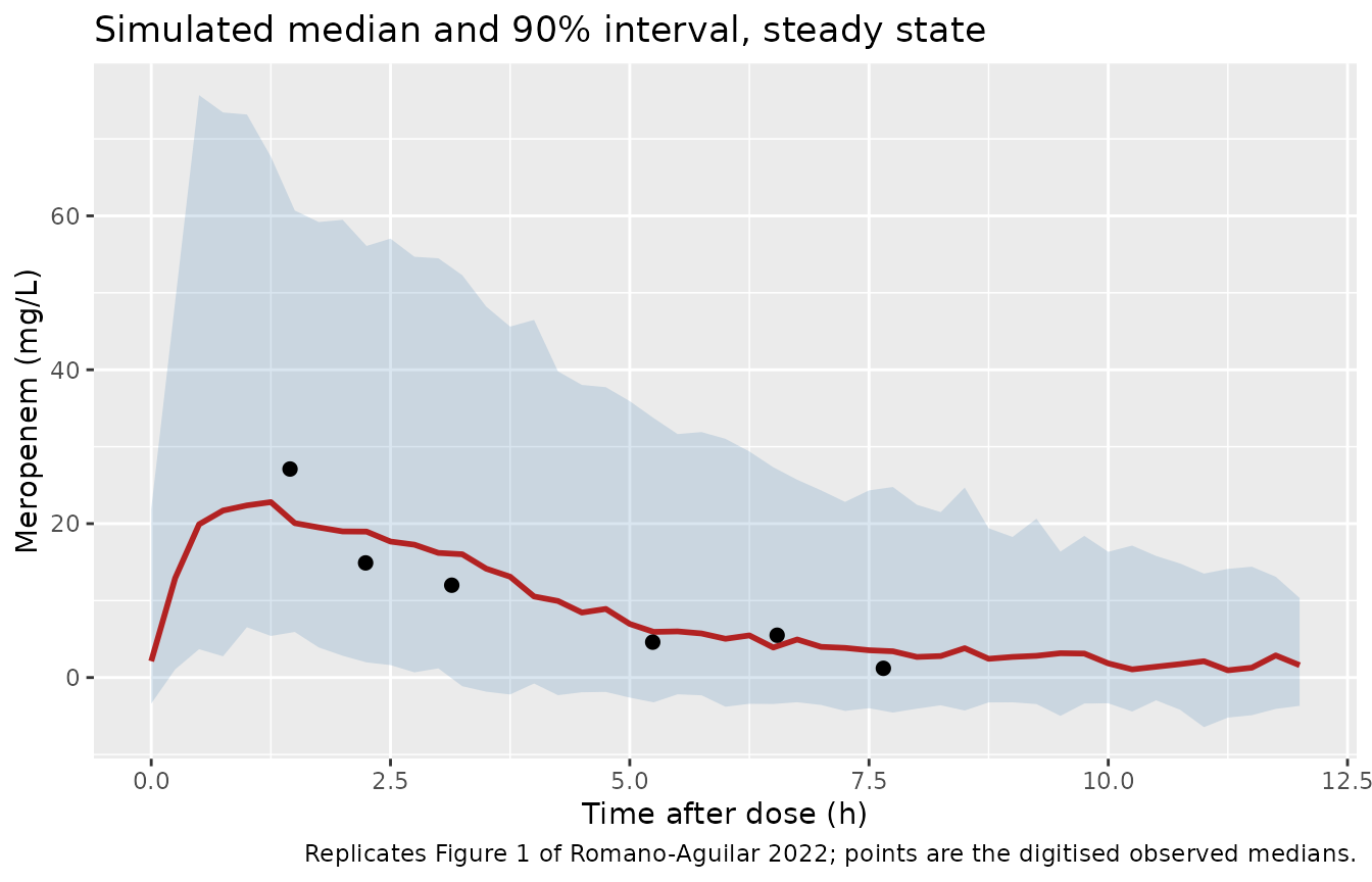
The observed median line in Figure 1 joins bin medians over sparse, mixed regimens. It is therefore compared with the simulated median only at the three nominal sampling times, 1, 3 and 6 h, within a factor of two.
sim_med <- sim |>
  dplyr::filter(time %in% c(1, 3, 6)) |>
  dplyr::group_by(time) |>
  dplyr::summarise(sim_median = median(sim), .groups = "drop") |>
  dplyr::mutate(fig1_median = stats::approx(fig1_median$time, fig1_median$conc,
                                            xout = time, rule = 2)$y,
                ratio = sim_median / fig1_median)

knitr::kable(
  sim_med |>
    dplyr::rename("Time after dose (h)" = time,
                  "Simulated median (mg/L)" = sim_median,
                  "Figure 1 observed median (mg/L)" = fig1_median,
                  "Ratio" = ratio),
  digits = 2,
  caption = "Simulated vs digitised observed median concentration."
)| Time after dose (h) | Simulated median (mg/L) | Figure 1 observed median (mg/L) | Ratio |
|---|---|---|---|
| 1 | 22.37 | 27.10 | 0.83 |
| 3 | 16.20 | 12.45 | 1.30 |
| 6 | 5.04 | 5.13 | 0.98 |
Probability of target attainment (Table 3)
Table 3 lists the initial regimens that achieve PTA > 90% for 50% and 100% fT>MIC at each creatinine clearance. The abstract does not state the MIC used. Each listed regimen is re-simulated below with 200 virtual patients at the stated creatinine clearance and steady state. The table reports the share of patients whose concentration (without residual error) exceeds the MIC for at least the target fraction of the interval, over a grid of MIC values.
tab3 <- read.csv(text = "
crcl,target,dose,tau,tinf
20,50,1000,24,0.5
20,50,500,12,0.5
20,50,500,8,0.5
40,50,500,12,2
40,50,1000,12,0.5
40,50,500,8,0.5
60,50,1000,12,3
60,50,1500,12,2
60,50,500,8,0.5
80,50,2000,12,3
80,50,500,8,3
80,50,1000,8,1
100,50,500,8,3
100,50,1000,8,2
120,50,1000,8,3
120,50,1500,8,2
120,50,500,6,2
140,50,1000,8,3
140,50,500,6,3
160,50,1500,8,3
160,50,500,6,3
180,50,500,6,3
180,50,1500,6,2
20,100,500,12,0.5
20,100,500,6,0.5
40,100,1000,8,2
40,100,1500,8,0.5
40,100,500,6,0.5
60,100,1000,6,3
60,100,1500,6,2")
tab3$row <- seq_len(nrow(tab3))
mics <- c(1, 2, 4)
n_pta <- 200
grid_frac <- seq(0, 1, by = 0.02)

ev_pta <- do.call(rbind, lapply(tab3$row, function(r) {
  p <- tab3[r, ]
  ids <- (r - 1) * n_pta + seq_len(n_pta)
  rbind(
    data.frame(id = ids, time = 0, amt = p$dose, rate = p$dose / p$tinf,
               ii = p$tau, ss = 1, evid = 1, cmt = "central", CRCL = p$crcl,
               row = r),
    data.frame(id = rep(ids, each = length(grid_frac)),
               time = rep(grid_frac * p$tau, n_pta), amt = 0, rate = 0, ii = 0,
               ss = 0, evid = 0, cmt = "central", CRCL = p$crcl, row = r)
  )
}))

rxode2::rxSetSeed(2022611)
sim_pta <- rxode2::rxSolve(ui, ev_pta, returnType = "data.frame", keep = "row",
                           maxsteps = 1e6)

pta <- do.call(rbind, lapply(mics, function(m) {
  sim_pta |>
    dplyr::group_by(row, id) |>
    dplyr::summarise(ft = mean(Cc > m), .groups = "drop") |>
    dplyr::left_join(tab3, by = "row") |>
    dplyr::group_by(row) |>
    dplyr::summarise(pta = mean(ft >= target / 100 - 1e-9), .groups = "drop") |>
    dplyr::mutate(mic = m)
})) |>
  dplyr::left_join(tab3, by = "row") |>
  dplyr::mutate(regimen = sprintf("%g mg q%gh over %g h", dose, tau, tinf),
                mic = paste0("PTA at MIC ", mic, " mg/L (%)"),
                pta = 100 * pta) |>
  dplyr::select(crcl, target, regimen, mic, pta) |>
  tidyr::pivot_wider(names_from = mic, values_from = pta)

knitr::kable(
  pta |>
    dplyr::rename("CLCr (mL/min/1.73 m^2)" = crcl,
                  "fT>MIC target (%)" = target,
                  "Table 3 regimen" = regimen),
  digits = 0,
  caption = "Simulated PTA of every Table 3 regimen (Table 3 lists them as PTA > 90%)."
)| CLCr (mL/min/1.73 m^2) | fT>MIC target (%) | Table 3 regimen | PTA at MIC 1 mg/L (%) | PTA at MIC 2 mg/L (%) | PTA at MIC 4 mg/L (%) |
|---|---|---|---|---|---|
| 20 | 50 | 1000 mg q24h over 0.5 h | 98 | 94 | 86 |
| 20 | 50 | 500 mg q12h over 0.5 h | 100 | 100 | 97 |
| 20 | 50 | 500 mg q8h over 0.5 h | 100 | 100 | 100 |
| 40 | 50 | 500 mg q12h over 2 h | 94 | 90 | 78 |
| 40 | 50 | 1000 mg q12h over 0.5 h | 96 | 94 | 87 |
| 40 | 50 | 500 mg q8h over 0.5 h | 99 | 98 | 94 |
| 60 | 50 | 1000 mg q12h over 3 h | 96 | 92 | 86 |
| 60 | 50 | 1500 mg q12h over 2 h | 98 | 93 | 84 |
| 60 | 50 | 500 mg q8h over 0.5 h | 94 | 86 | 74 |
| 80 | 50 | 2000 mg q12h over 3 h | 94 | 90 | 84 |
| 80 | 50 | 500 mg q8h over 3 h | 98 | 94 | 74 |
| 80 | 50 | 1000 mg q8h over 1 h | 97 | 92 | 85 |
| 100 | 50 | 500 mg q8h over 3 h | 97 | 88 | 64 |
| 100 | 50 | 1000 mg q8h over 2 h | 92 | 88 | 75 |
| 120 | 50 | 1000 mg q8h over 3 h | 96 | 92 | 72 |
| 120 | 50 | 1500 mg q8h over 2 h | 90 | 88 | 78 |
| 120 | 50 | 500 mg q6h over 2 h | 92 | 86 | 63 |
| 140 | 50 | 1000 mg q8h over 3 h | 97 | 89 | 68 |
| 140 | 50 | 500 mg q6h over 3 h | 100 | 92 | 68 |
| 160 | 50 | 1500 mg q8h over 3 h | 93 | 88 | 78 |
| 160 | 50 | 500 mg q6h over 3 h | 100 | 92 | 62 |
| 180 | 50 | 500 mg q6h over 3 h | 98 | 88 | 44 |
| 180 | 50 | 1500 mg q6h over 2 h | 93 | 90 | 78 |
| 20 | 100 | 500 mg q12h over 0.5 h | 96 | 91 | 80 |
| 20 | 100 | 500 mg q6h over 0.5 h | 100 | 100 | 100 |
| 40 | 100 | 1000 mg q8h over 2 h | 96 | 92 | 84 |
| 40 | 100 | 1500 mg q8h over 0.5 h | 96 | 90 | 84 |
| 40 | 100 | 500 mg q6h over 0.5 h | 95 | 90 | 80 |
| 60 | 100 | 1000 mg q6h over 3 h | 96 | 93 | 84 |
| 60 | 100 | 1500 mg q6h over 2 h | 98 | 96 | 91 |
pta2 <- pta[["PTA at MIC 2 mg/L (%)"]]
pta4 <- pta[["PTA at MIC 4 mg/L (%)"]]
cat(sprintf("median PTA across Table 3 rows: %.0f%% at MIC 2 mg/L, %.0f%% at MIC 4 mg/L\n",
            median(pta2), median(pta4)))
#> median PTA across Table 3 rows: 92% at MIC 2 mg/L, 80% at MIC 4 mg/L
# Table 3's regimens sit at the 90% boundary for an MIC of about 2 mg/L: the
# median row is near 90% there and well below it at 4 mg/L. A two-fold error
# in clearance or volume moves the median row PTA at 2 mg/L away from 90% by
# far more than the +/- 7 points allowed here.
stopifnot(abs(median(pta2) - 91) < 7, median(pta4) < 85)
The listed regimens cluster at the 90% boundary for an MIC of 2 mg/L, which is consistent with the abstract’s simulations having used that MIC (the EUCAST clinical breakpoint for Enterobacterales and Pseudomonas aeruginosa).
For augmented renal clearance and the 100% fT>MIC target the
abstract recommends continuous infusion, because no intermittent regimen
reached PTA > 90%. The typical steady-state concentration of a
continuous infusion is daily dose / 24 / CL:
ci <- expand.grid(daily = c(3000, 6000), CRCL = c(80, 130, 180, 240)) |>
  dplyr::mutate(cl = 11.9 * CRCL / 102.23, css = daily / 24 / cl)
knitr::kable(
  ci |>
    dplyr::select(daily, CRCL, cl, css) |>
    dplyr::rename("Daily dose (mg)" = daily,
                  "CLCr (mL/min/1.73 m^2)" = CRCL,
                  "Typical CL (L/h)" = cl,
                  "Typical Css (mg/L)" = css),
  digits = c(0, 0, 2, 2),
  caption = "Typical continuous-infusion steady-state concentrations."
)| Daily dose (mg) | CLCr (mL/min/1.73 m^2) | Typical CL (L/h) | Typical Css (mg/L) |
|---|---|---|---|
| 3000 | 80 | 9.31 | 13.42 |
| 6000 | 80 | 9.31 | 26.85 |
| 3000 | 130 | 15.13 | 8.26 |
| 6000 | 130 | 15.13 | 16.52 |
| 3000 | 180 | 20.95 | 5.97 |
| 6000 | 180 | 20.95 | 11.93 |
| 3000 | 240 | 27.94 | 4.47 |
| 6000 | 240 | 27.94 | 8.95 |
PKNCA validation
Non-compartmental analysis over one steady-state interval of the two
most common regimens, 1000 mg q8h over 0.5 h and over 3 h, in 200
patients each drawn from the same creatinine clearance distribution. At
steady state the interval AUC must equal Dose / CL for
every subject. The abstract reports no NCA of its own.
set.seed(8)
nca_regimens <- data.frame(treatment = c("1000 mg q8h, 0.5 h", "1000 mg q8h, 3 h"),
                           tinf = c(0.5, 3))
nca_cohort <- do.call(rbind, lapply(seq_len(nrow(nca_regimens)), function(j) {
  data.frame(id = (j - 1) * n_sub + seq_len(n_sub),
             treatment = nca_regimens$treatment[j],
             tinf = nca_regimens$tinf[j],
             CRCL = draw_crcl(n_sub))
}))
nca_t <- sort(unique(c(seq(0, 3, by = 0.1), seq(3.25, 8, by = 0.25))))
ev_nca <- do.call(rbind, lapply(seq_len(nrow(nca_cohort)), function(i) {
  p <- nca_cohort[i, ]
  rbind(
    data.frame(id = p$id, time = 0, amt = 1000, rate = 1000 / p$tinf, ii = 8,
               ss = 1, evid = 1, cmt = "central", CRCL = p$CRCL,
               treatment = p$treatment),
    data.frame(id = p$id, time = nca_t, amt = 0, rate = 0, ii = 0, ss = 0,
               evid = 0, cmt = "central", CRCL = p$CRCL, treatment = p$treatment)
  )
}))

# Tight tolerances: at the highest creatinine clearances the trough falls to
# a level where default absolute tolerance can return slightly negative
# concentrations, which PKNCA's log-down trapezoid cannot integrate.
rxode2::rxSetSeed(8)
sim_nca <- rxode2::rxSolve(ui, ev_nca, returnType = "data.frame",
                           keep = "treatment", maxsteps = 1e6,
                           rtol = 1e-10, atol = 1e-12, ssRtol = 1e-10, ssAtol = 1e-12)
stopifnot(min(sim_nca$Cc) >= 0)

conc <- sim_nca |>
  dplyr::filter(!is.na(Cc)) |>
  dplyr::select(id, time, Cc, treatment)
dose_df <- ev_nca |>
  dplyr::filter(evid == 1) |>
  dplyr::select(id, time, amt, treatment)

o_conc <- PKNCA::PKNCAconc(conc, Cc ~ time | treatment + id)
o_dose <- PKNCA::PKNCAdose(dose_df, amt ~ time | treatment + id)
intervals <- data.frame(start = 0, end = 8, cmax = TRUE, tmax = TRUE, cmin = TRUE,
                        auclast = TRUE, cav = TRUE)
nca <- PKNCA::pk.nca(PKNCA::PKNCAdata(o_conc, o_dose, intervals = intervals))
nca_res <- as.data.frame(nca$result)

nca_summary <- nca_res |>
  dplyr::group_by(treatment, PPTESTCD) |>
  dplyr::summarise(median = median(PPORRES), .groups = "drop") |>
  tidyr::pivot_wider(names_from = PPTESTCD, values_from = median)

knitr::kable(
  nca_summary |>
    dplyr::select(treatment, cmax, tmax, cmin, auclast, cav) |>
    dplyr::rename("Regimen" = treatment, "Cmax (mg/L)" = cmax, "Tmax (h)" = tmax,
                  "Cmin (mg/L)" = cmin, "AUC0-8 (mg*h/L)" = auclast,
                  "Cavg (mg/L)" = cav),
  digits = 2,
  caption = "Median steady-state NCA parameters (simulated, individual predictions)."
)| Regimen | Cmax (mg/L) | Tmax (h) | Cmin (mg/L) | AUC0-8 (mg*h/L) | Cavg (mg/L) |
|---|---|---|---|---|---|
| 1000 mg q8h, 0.5 h | 37.47 | 0.5 | 1.18 | 89.82 | 11.23 |
| 1000 mg q8h, 3 h | 22.19 | 3.0 | 2.59 | 85.96 | 10.74 |
auc_chk <- nca_res |>
  dplyr::filter(PPTESTCD == "auclast") |>
  dplyr::left_join(sim_nca |> dplyr::distinct(id, cl), by = "id") |>
  dplyr::mutate(rel_err = PPORRES * cl / 1000 - 1)

cat(sprintf("AUC0-8 x CL / Dose - 1: median %.2g, 90th pct |err| %.2g\n",
            median(auc_chk$rel_err), quantile(abs(auc_chk$rel_err), 0.9)))
#> AUC0-8 x CL / Dose - 1: median -0.0001, 90th pct |err| 0.00063
# Trapezoidal error on a 0.1-0.25 h grid is small for typical half-lives; a
# wrong clearance, dose or infusion rate moves this by tens of percent.
stopifnot(abs(median(auc_chk$rel_err)) < 0.01,
          quantile(abs(auc_chk$rel_err), 0.9) < 0.05)
Assumptions and deviations
-
Variance scale of the interindividual variability.
Table 2 prints both terms as CV% under an omega-squared symbol and does
not say how CV% was computed. The log-normal conversion
omega^2 = log(1 + CV^2)is used, giving variances of 0.2745 (CL) and 0.1996 (V). The alternative readingomega^2 = CV^2(0.316 and 0.221) cannot be ruled out from the abstract: the bootstrap columns are percentile intervals, which do not discriminate the two, and the Table 3 PTA values change by at most a few percentage points between the readings. - Residual error. Table 2 reports one residual term, sigma = 3.53 in ug/mL, with no description of the error model. A value in concentration units is read as an additive standard deviation.
- Covariate reference. The Results print the reference as 102.23 and Table 2 as 102; 102.23 is used. The abstract does not say which cohort statistic it is (the Table 1 median is 103.14).
-
Cockcroft-Gault details. The body weight entering
the Cockcroft-Gault formula and the normalisation to 1.73 m^2 are not
described.
CRCLshould be supplied in mL/min/1.73 m^2 as in Table 1. Clearance is linear inCRCLthrough the origin with no cap, so it approaches zero for anuric patients; the model was fitted to 13.5-241.4 mL/min/1.73 m^2. - Virtual cohort. Creatinine clearance is drawn log-normally around the Table 1 median within the observed range, and the regimen from the three Table 1 marginal frequencies independently. The real pairing of doses, intervals and infusion times is not reported. Steady state is assumed at sampling.
- Figure 1 digitisation. The observed median line was read at its vertices from the image; precision is about +/- 1 mg/L.
- MIC in Table 3. The abstract does not state the MIC used for its PTA simulations. The re-simulation reports a grid of MICs; the regimens sit at the 90% boundary for 2 mg/L. Whether the abstract’s simulations included residual error is not stated; the re-simulation excludes it.
- Protein binding. The abstract states its targets as %t > MIC on total concentration; meropenem binding is low (about 2%), and total concentrations are used.
- Interindividual variability correlation. No covariance between the CL and V random effects is reported; they are independent.