Model and source
- Citation: Nie Y, Sun X, Cao R, Tang S, Zhou Q, Zhou M, Chen Z, Huang S. Population pharmacokinetic of epidural sufentanil in labouring women: a multicentric, prospective, observational study. Drug Des Devel Ther. 2025;19:971-980. doi:10.2147/DDDT.S500189.
- Description: Two-compartment population PK model of epidural
sufentanil in labouring women (Nie 2025; N = 41 primiparous women
receiving sufentanil 0.3 ug/mL with 0.1% ropivacaine by
patient-controlled epidural analgesia at six Chinese centres).
Compartment 1 is the maternal central compartment and compartment 2 is
the umbilical cord (placental circulation) compartment; the two exchange
through a slow inter-compartmental clearance CL2. The epidural
compartment could not be estimated from the sparse data and was assumed
to have merged with the central compartment, so doses enter
centraldirectly and CL / V1 are apparent values (bioavailability assumed 1). Cord equilibration is far slower than maternal elimination (K21 = CL2/V2 gives a cord half-life of ~9.7 h against a ~2.0 h maternal elimination half-life), which reproduces the paper’s central finding that umbilical cord concentrations decline only slowly once the epidural infusion is stopped. Inter-individual variability was estimated on CL and V1 only; IIV on CL2 and V2 did not improve the fit and was excluded. Residual error is proportional with a separate magnitude for maternal and umbilical cord observations. - Article: https://doi.org/10.2147/DDDT.S500189
This is the first published population PK model of epidural sufentanil in labouring women. Its purpose is not maternal exposure – which is very low – but the quantification of placental transfer: the model carries an explicit umbilical cord compartment so that fetal-side exposure can be predicted at, and after, delivery.
Population
Forty-one primiparous women contributed to the final population PK analysis, a subset of the 90 parturients recruited between November 2018 and February 2019 across six Chinese centres (Nie 2025 Results, “Patient Characteristics”). They were 27.2 +/- 2.9 years old and weighed 70.2 +/- 7.5 kg, with ASA physical status II-III, BMI 18.5-30 kg/m^2, a singleton pregnancy and cervical dilation of 2 <= phi < 6 cm at the time of analgesia.
The analysis dataset held 79 maternal central-compartment concentrations and 37 umbilical cord concentrations. Maternal venous samples were scheduled at 0.5 h and 1 h after the epidural loading dose, at delivery, and 2 h after delivery; a single umbilical venous sample was drawn immediately after cord clamping. Not all four maternal samples were mandatory, so the design is sparse and unbalanced. Sufentanil was assayed by LC-MS/MS with a lower limit of quantification of 1 pg/mL.
No covariate model was reported. Nie 2025 Table 1 contains
structural, inter-individual-variability and residual rows only, and the
paper describes no covariate screening step, so the packaged model
carries no covariateData.
The same information is available programmatically via
readModelDb("Nie_2025_sufentanil")()$population.
pop <- rxode2::rxode(readModelDb("Nie_2025_sufentanil"))$population
#> ℹ parameter labels from comments will be replaced by 'label()'
str(pop[c("species", "n_subjects", "n_studies", "age_mean", "weight_mean")])
#> List of 5
#>  $ species    : chr "human"
#>  $ n_subjects : int 41
#>  $ n_studies  : int 1
#>  $ age_mean   : chr "27.2 +/- 2.9 years"
#>  $ weight_mean: chr "70.2 +/- 7.5 kg"
Source trace
Every ini() entry in
inst/modeldb/specificDrugs/Nie_2025_sufentanil.R carries an
in-file comment naming its origin. They are collected here for
review.
| Equation / parameter | Value | Source location |
|---|---|---|
lcl (CL) |
176 L/h (RSE 9.25%) | Table 1, “Structural parameters” |
lvc (V1) |
519 L (RSE 6.45%) | Table 1, “Structural parameters” |
lqcord (CL2) |
0.0134 L/h (RSE 43.2%) | Table 1, “Structural parameters” |
lvcord (V2) |
0.187 L (RSE 39.9%) | Table 1, “Structural parameters” |
etalcl |
0.255046 = log(0.539^2 + 1) | Table 1, “IIV of CL” = 53.9 %CV (RSE 12%) |
etalvc |
0.046429 = log(0.218^2 + 1) | Table 1, “IIV of V1” = 21.8 %CV (RSE 26.9%) |
propSd |
0.206 | Table 1, “eps prop1 (%)” = 20.6% (RSE 13.4%) |
propSd_Ccord |
0.355 | Table 1, “eps prop2 (%)” = 35.5% (RSE 12%) |
kel <- cl / vc |
n/a | Methods, “Sufentanil Structural Pharmacokinetic Model”: K10 = CL/V1 |
k12 <- qcord / vc |
n/a | Methods, same section: K12 = CL2/V1 |
k21 <- qcord / vcord |
n/a | Methods, same section: K21 = CL2/V2 |
d/dt(central), d/dt(cord)
|
n/a | Methods, same section (A1, A2 mass balance); Figure 1 schematic |
Dose enters central
|
n/a | Methods, same section: the epidural compartment “merged with the central compartment” |
| Exponential IIV, log-normal | n/a | Methods, “Population PK Model Development” |
| Proportional-only residual | n/a | Methods, same section: “eps_add was removed due to its lesser significance” |
The IIV magnitudes in Table 1 are reported as %CV, so the internal
variances are omega^2 = log(CV^2 + 1). That the conversion
round-trips is asserted below.
ui <- rxode2::rxode(readModelDb("Nie_2025_sufentanil"))
#> ℹ parameter labels from comments will be replaced by 'label()'
omegas <- c(etalcl = 0.255046, etalvc = 0.046429)
roundtrip <- sqrt(exp(omegas) - 1) * 100
stopifnot(abs(roundtrip - c(53.9, 21.8)) < 0.05)
round(roundtrip, 2)
#> etalcl etalvc
#>   53.9   21.8
Dosing regimen
The protocol (Nie 2025 Methods, “Anesthesia Management”) is a 5 mL epidural injection of the study mixture, a 10 mL bolus five minutes later, and patient-controlled epidural analgesia from 30 min with a 6 mL/h continuous infusion, a 6 mL demand bolus and a 15 min lockout, maintained until delivery.
The sufentanil concentration of that mixture is reported inconsistently: the Abstract states 0.3 ug/mL, while the Methods state 3 ug/mL. The two differ tenfold, and the model’s own parameters settle it. At 6 mL/h the steady-state maternal concentration is the infusion rate divided by CL:
CL <- 176; V1 <- 519; CL2 <- 0.0134; V2 <- 0.187
falsifier <- tibble::tibble(
  mixture_ug_per_mL = c(0.3, 3),
  css_pg_per_mL     = mixture_ug_per_mL * 6 * 1000 / CL,
  loading_c0_pg_per_mL = mixture_ug_per_mL * 15 * 1000 / V1
)
falsifier |>
  dplyr::rename(
    "Mixture (ug/mL)"                  = mixture_ug_per_mL,
    "Maternal Css at 6 mL/h (pg/mL)"   = css_pg_per_mL,
    "C0 after the 15 mL loading (pg/mL)" = loading_c0_pg_per_mL
  ) |>
knitr::kable(digits = 1, caption = "Which mixture concentration is consistent with Table 1?")| Mixture (ug/mL) | Maternal Css at 6 mL/h (pg/mL) | C0 after the 15 mL loading (pg/mL) |
|---|---|---|
| 0.3 | 10.2 | 8.7 |
| 3.0 | 102.3 | 86.7 |
Observed maternal concentrations in Nie 2025 Figure 2 (left panel) span roughly 3-30 pg/mL, with the 0.5-1 h loading cluster around 5-15 pg/mL. Only the 0.3 ug/mL mixture reproduces that; 3 ug/mL predicts a plateau of ~102 pg/mL, which is above every observed point in the paper. This vignette therefore uses 0.3 ug/mL and treats the Methods figure as a typographical error. 0.3 ug/mL is also the clinically conventional strength for epidural labour analgesia.
MIX_UG_PER_ML <- 0.3       # sufentanil concentration of the epidural mixture
LOAD1  <- 5  * MIX_UG_PER_ML * 1000   # ng, 5 mL initial injection at t = 0
LOAD2  <- 10 * MIX_UG_PER_ML * 1000   # ng, 10 mL bolus at t = 5 min
T_LOAD2 <- 5 / 60                     # h
T_PCEA  <- 0.5                        # h, PCEA started 30 min after loading
INF_RATE <- 6 * MIX_UG_PER_ML * 1000  # ng/h, 6 mL/h continuous infusion
LLOQ <- 1                             # pg/mL (Methods, assay section)
c(LOAD1 = LOAD1, LOAD2 = LOAD2, INF_RATE = INF_RATE)
#>    LOAD1    LOAD2 INF_RATE
#>     1500     3000     1800
Amounts are in ng and volumes in L, so amount / volume
is ng/L, which is identical to the pg/mL used throughout the paper. No
conversion constant is needed anywhere in the model.
Virtual cohort
Original observed data are not available. Two virtual cohorts are used, each well under the 200-per-arm cap.
- Typical-value profile – one subject with the random effects zeroed, on a dense time grid, to reproduce the shape of the individual fits in Figure 4.
- Figure 2 cohort – 200 women sampled exactly as the trial sampled them (maternal at 0.5 h, 1 h, delivery and delivery + 2 h; a single cord sample at delivery), with each woman’s delivery time drawn over the 2.5-10.5 h range spanned by the observed sampling times in Figure 2.
set.seed(20250213)
N_COHORT <- 200

subj <- tibble::tibble(
  id       = seq_len(N_COHORT),
  delivery = runif(N_COHORT, 2.5, 10.5)   # h, epidural infusion stops at delivery
)

# Dosing is identical for everyone except the infusion duration, which runs from
# T_PCEA until that woman's delivery. `rate` + `amt` encodes the zero-order
# infusion; `delivery` rides along so rxSolve(keep = ) can return it.
dosing <- dplyr::bind_rows(
  subj |> dplyr::transmute(id, delivery, time = 0, amt = LOAD1, rate = 0,
                           evid = 1L, cmt = "central"),
  subj |> dplyr::transmute(id, delivery, time = T_LOAD2, amt = LOAD2, rate = 0,
                           evid = 1L, cmt = "central"),
  subj |> dplyr::transmute(id, delivery, time = T_PCEA,
                           amt = INF_RATE * (delivery - T_PCEA), rate = INF_RATE,
                           evid = 1L, cmt = "central")
)

# Observation rows use the DECLARED endpoint names (`Cc`, `Ccord`). This model
# declares two endpoints, so rxode2 allocates a slot for each and the event
# table must say which endpoint a row belongs to; using an ODE state name here
# instead raises "'dvid'->'cmt' on observation record".
obs <- dplyr::bind_rows(
  subj |> tidyr::crossing(t_fixed = c(0.5, 1)) |>
    dplyr::transmute(id, delivery, time = t_fixed, amt = NA_real_, rate = 0,
                     evid = 0L, cmt = "Cc"),
  subj |> dplyr::transmute(id, delivery, time = delivery, amt = NA_real_, rate = 0,
                           evid = 0L, cmt = "Cc"),
  subj |> dplyr::transmute(id, delivery, time = delivery + 2, amt = NA_real_, rate = 0,
                           evid = 0L, cmt = "Cc"),
  subj |> dplyr::transmute(id, delivery, time = delivery, amt = NA_real_, rate = 0,
                           evid = 0L, cmt = "Ccord")
)

events <- dplyr::bind_rows(dosing, obs) |>
  dplyr::arrange(id, time, dplyr::desc(evid)) |>
  as.data.frame()

stopifnot(!anyDuplicated(unique(events[, c("id", "time", "evid", "cmt")])))
nrow(events)
#> [1] 1600
Simulation
useLinCmt = FALSE is required: rxode2’s automatic
ODE-to-linCmt() conversion corrupts the
endpoint-to-compartment mapping for multi-output models of this
shape.
mod <- readModelDb("Nie_2025_sufentanil")

sim_cohort <- rxode2::rxSolve(
  mod, events = events, keep = "delivery", useLinCmt = FALSE
) |>
  as.data.frame()
#> ℹ parameter labels from comments will be replaced by 'label()'

# CMT 3 is the maternal endpoint (Cc), CMT 4 the umbilical cord endpoint
# (Ccord). `Cc` / `Ccord` are the individual predictions; `sim` carries the
# proportional residual error and is the simulated *observation*.
sim_cohort <- sim_cohort |>
  dplyr::mutate(
    endpoint = dplyr::if_else(CMT == 3, "Maternal plasma", "Umbilical cord"),
    ipred    = dplyr::if_else(CMT == 3, Cc, Ccord)
  )

stopifnot(dplyr::n_distinct(sim_cohort$id) == N_COHORT)
The typical-value profile uses a fixed 8 h infusion – a representative labour duration inside the observed range – on a dense grid.
grid_dense <- c(seq(0, 12, by = 0.05), seq(12.25, 48, by = 0.25))
INF_DUR <- 8

ev_typ <- rxode2::et(amt = LOAD1, time = 0, cmt = "central") |>
  rxode2::et(amt = LOAD2, time = T_LOAD2, cmt = "central") |>
  rxode2::et(amt = INF_RATE * INF_DUR, time = T_PCEA, dur = INF_DUR, cmt = "central") |>
  rxode2::et(grid_dense, cmt = "Cc") |>
  rxode2::et(grid_dense, cmt = "Ccord")

sim_typ <- rxode2::rxSolve(rxode2::zeroRe(mod), events = ev_typ, useLinCmt = FALSE) |>
  as.data.frame() |>
  dplyr::filter(CMT == 3)   # both Cc and Ccord are returned on every row
#> ℹ parameter labels from comments will be replaced by 'label()'
#> ℹ omega/sigma items treated as zero: 'etalcl', 'etalvc'
Replicate published figures
Figure 4 – individual fits: maternal falls fast, cord does not
Figure 4 of Nie 2025 shows, for each woman, a maternal profile (solid black) that plateaus during the epidural infusion and then falls steeply once the infusion stops at delivery, alongside a cord profile (dashed red) that rises slowly throughout labour and then stays almost flat. The typical-value prediction reproduces both.
sim_typ |>
  dplyr::select(time, `Maternal plasma` = Cc, `Umbilical cord` = Ccord) |>
  tidyr::pivot_longer(-time, names_to = "endpoint", values_to = "conc") |>
  dplyr::filter(conc > 0) |>
  ggplot(aes(time, conc, colour = endpoint, linetype = endpoint)) +
  geom_vline(xintercept = T_PCEA + INF_DUR, linetype = "dotted") +
  geom_line(linewidth = 0.9) +
  annotate("text", x = T_PCEA + INF_DUR + 0.4, y = 0.02,
           label = "infusion stops (delivery)", hjust = 0, size = 3) +
  scale_y_log10() +
  scale_colour_manual(values = c("Maternal plasma" = "black", "Umbilical cord" = "red")) +
  labs(x = "Time (h)", y = "Sufentanil concentration (pg/mL)",
       colour = NULL, linetype = NULL,
       title = "Typical-value maternal and umbilical cord profiles",
       caption = "Replicates the shape of Figure 4 of Nie 2025 (8 h infusion).")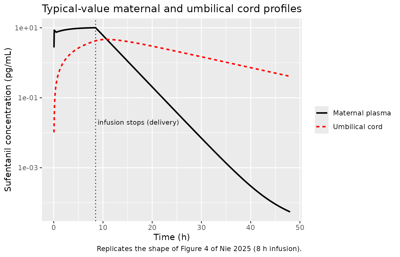
The paper’s qualitative claims are asserted numerically below.
at_time <- function(tt, col) sim_typ[[col]][which.min(abs(sim_typ$time - tt))]
t_stop <- T_PCEA + INF_DUR

cord_peak_time <- sim_typ$time[which.max(sim_typ$Ccord)]
fig4 <- tibble::tibble(
  claim = c(
    "Maternal plateau during infusion (pg/mL)",
    "Cord concentration at delivery (pg/mL)",
    "Cord peaks AFTER the infusion stops (h past stop)",
    "Maternal concentration 16 h after stop (pg/mL)",
    "Cord concentration 16 h after stop, as % of its peak"
  ),
  value = c(
    at_time(t_stop, "Cc"),
    at_time(t_stop, "Ccord"),
    cord_peak_time - t_stop,
    at_time(t_stop + 16, "Cc"),
    100 * at_time(t_stop + 16, "Ccord") / max(sim_typ$Ccord)
  )
)

# The paper's central finding: the cord compartment keeps filling after the
# infusion stops, and is still near its peak when maternal drug has gone.
stopifnot(cord_peak_time > t_stop)
stopifnot(at_time(t_stop + 16, "Cc") < 0.1)
stopifnot(100 * at_time(t_stop + 16, "Ccord") / max(sim_typ$Ccord) > 40)

fig4 |>
  dplyr::rename("Claim from Nie 2025" = claim, "Simulated" = value) |>
knitr::kable(digits = 3, caption = "Numerical restatement of the Figure 4 narrative.")| Claim from Nie 2025 | Simulated |
|---|---|
| Maternal plateau during infusion (pg/mL) | 10.043 |
| Cord concentration at delivery (pg/mL) | 4.235 |
| Cord peaks AFTER the infusion stops (h past stop) | 2.300 |
| Maternal concentration 16 h after stop (pg/mL) | 0.044 |
| Cord concentration 16 h after stop, as % of its peak | 47.174 |
Figure 2 – observed concentration-time scatter
Figure 2 plots every observed concentration against time, maternal on the left and umbilical cord on the right. Simulating the trial’s own sparse sampling design reproduces both clouds. Simulated observations below the 1 pg/mL assay limit are dropped, as they would have been in the real dataset.
sim_obs <- sim_cohort |>
  dplyr::filter(sim >= LLOQ)

ggplot(sim_obs, aes(time, sim)) +
  geom_point(shape = 1, alpha = 0.5) +
  facet_wrap(~endpoint) +
  scale_y_log10(limits = c(0.2, 60)) +
  labs(x = "Time (h)", y = "Sufentanil concentration (pg/mL)",
       title = "Simulated concentrations under the trial's sampling design",
       caption = "Replicates Figure 2 of Nie 2025 (left: maternal; right: umbilical cord).")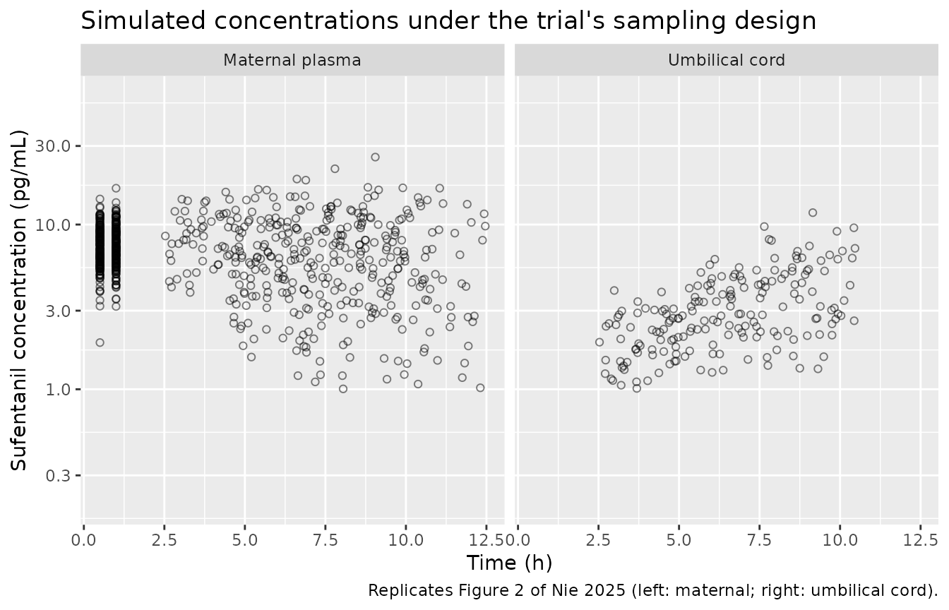
# Ranges read off the log axis of Nie 2025 Figure 2 by the maintainers
# (graphical digitisation, not a printed table). Used only as a validation
# envelope -- no model parameter is derived from them.
observed_envelope <- tibble::tribble(
  ~endpoint,          ~obs_low, ~obs_high,
  "Maternal plasma",  3,        30,
  "Umbilical cord",   0.6,      10
)

sim_obs |>
  dplyr::group_by(endpoint) |>
  dplyr::summarise(
    sim_p05 = quantile(sim, 0.05),
    sim_p50 = quantile(sim, 0.50),
    sim_p95 = quantile(sim, 0.95),
    .groups = "drop"
  ) |>
  dplyr::left_join(observed_envelope, by = "endpoint") |>
  dplyr::rename(
    "Endpoint"                        = endpoint,
    "Simulated 5th pctile (pg/mL)"    = sim_p05,
    "Simulated median (pg/mL)"        = sim_p50,
    "Simulated 95th pctile (pg/mL)"   = sim_p95,
    "Figure 2 observed low (pg/mL)"   = obs_low,
    "Figure 2 observed high (pg/mL)"  = obs_high
  ) |>
knitr::kable(digits = 2, caption = "Simulated spread vs the observed envelope of Figure 2.")| Endpoint | Simulated 5th pctile (pg/mL) | Simulated median (pg/mL) | Simulated 95th pctile (pg/mL) | Figure 2 observed low (pg/mL) | Figure 2 observed high (pg/mL) |
|---|---|---|---|---|---|
| Maternal plasma | 2.33 | 7.04 | 12.80 | 3.0 | 30 |
| Umbilical cord | 1.31 | 2.79 | 6.77 | 0.6 | 10 |
Fetal-to-maternal ratio at delivery
The paper contrasts its model-based transfer estimate with the single-timepoint fetomaternal (F/M) ratio of 0.81 reported for epidural sufentanil in an earlier study (Nie 2025 Discussion, reference 10), arguing that F/M ratios overstate fetal exposure because the cord compartment is still filling at delivery.
fm <- dplyr::inner_join(
  sim_cohort |> dplyr::filter(CMT == 3, abs(time - delivery) < 1e-9) |>
    dplyr::select(id, maternal = ipred),
  sim_cohort |> dplyr::filter(CMT == 4) |> dplyr::select(id, cord = ipred),
  by = "id"
) |>
  dplyr::mutate(ratio = cord / maternal)

stopifnot(nrow(fm) == N_COHORT)
tibble::tibble(
  quantity = c("Simulated F/M ratio at delivery, median",
               "Simulated F/M ratio at delivery, 5th-95th pctile",
               "Literature F/M ratio cited by Nie 2025 (reference 10)"),
  value = c(sprintf("%.2f", median(fm$ratio)),
            sprintf("%.2f - %.2f", quantile(fm$ratio, 0.05), quantile(fm$ratio, 0.95)),
            "0.81")
) |>
  dplyr::rename("Quantity" = quantity, "Value" = value) |>
knitr::kable(caption = "Model-predicted placental transfer at delivery.")| Quantity | Value |
|---|---|
| Simulated F/M ratio at delivery, median | 0.33 |
| Simulated F/M ratio at delivery, 5th-95th pctile | 0.18 - 0.51 |
| Literature F/M ratio cited by Nie 2025 (reference 10) | 0.81 |
The simulated median of ~0.3 sits well below the cited 0.81 and matches the cord / maternal separation drawn in Figure 4, supporting the paper’s argument.
PKNCA validation
NCA is run on the maternal endpoint over a dense grid. Nie 2025 reports no NCA table, so the comparison targets are the structural identities implied by Table 1 rather than published NCA values.
N_NCA <- 100
grid_nca <- c(seq(0, 12, by = 0.1), seq(12.5, 48, by = 0.5))

ev_nca <- rxode2::et(amt = LOAD1, time = 0, cmt = "central") |>
  rxode2::et(amt = LOAD2, time = T_LOAD2, cmt = "central") |>
  rxode2::et(amt = INF_RATE * INF_DUR, time = T_PCEA, dur = INF_DUR, cmt = "central") |>
  rxode2::et(grid_nca, cmt = "Cc") |>
  rxode2::et(id = seq_len(N_NCA))

set.seed(9876)
sim_nca_raw <- rxode2::rxSolve(mod, events = ev_nca, useLinCmt = FALSE) |>
  as.data.frame()

DOSE_TOTAL <- LOAD1 + LOAD2 + INF_RATE * INF_DUR

# Filter on !is.na(Cc) only -- a `time > 0` or `Cc > 0` filter would drop the
# time-zero anchor PKNCA needs for AUC.
sim_nca <- sim_nca_raw |>
  dplyr::filter(!is.na(Cc)) |>
  dplyr::mutate(treatment = "PCEA 0.3 ug/mL sufentanil") |>
  dplyr::select(id, time, Cc, treatment) |>
  dplyr::distinct(id, time, .keep_all = TRUE)

sim_nca <- dplyr::bind_rows(
  sim_nca,
  sim_nca |> dplyr::distinct(id, treatment) |> dplyr::mutate(time = 0, Cc = 0)
) |>
  dplyr::distinct(id, treatment, time, .keep_all = TRUE) |>
  dplyr::arrange(id, time)

stopifnot(nrow(sim_nca) > 0, all(sim_nca$Cc >= 0))

dose_df <- sim_nca |>
  dplyr::distinct(id, treatment) |>
  dplyr::mutate(time = 0, amt = DOSE_TOTAL)

conc_obj <- PKNCA::PKNCAconc(sim_nca, Cc ~ time | treatment + id)
dose_obj <- PKNCA::PKNCAdose(dose_df, amt ~ time | treatment + id)

intervals <- data.frame(
  start = 0, end = Inf,
  cmax = TRUE, tmax = TRUE, auclast = TRUE, aucinf.obs = TRUE, half.life = TRUE
)

nca_res <- suppressWarnings(
  PKNCA::pk.nca(PKNCA::PKNCAdata(conc_obj, dose_obj, intervals = intervals))
)

nca_tab <- as.data.frame(nca_res$result)
nca_tab |>
  dplyr::filter(PPTESTCD %in% c("cmax", "tmax", "auclast", "aucinf.obs", "half.life")) |>
  dplyr::group_by(PPTESTCD) |>
  dplyr::summarise(median = median(PPORRES, na.rm = TRUE),
                   p05 = quantile(PPORRES, 0.05, na.rm = TRUE),
                   p95 = quantile(PPORRES, 0.95, na.rm = TRUE),
                   .groups = "drop") |>
  dplyr::rename("NCA parameter" = PPTESTCD, "Median" = median,
                "5th pctile" = p05, "95th pctile" = p95) |>
knitr::kable(digits = 3, caption = "PKNCA summary of the simulated maternal profile.")| NCA parameter | Median | 5th pctile | 95th pctile |
|---|---|---|---|
| aucinf.obs | 107.975 | 52.206 | 206.548 |
| auclast | 107.975 | 52.206 | 206.362 |
| cmax | 10.971 | 7.407 | 16.446 |
| half.life | 5.840 | 2.644 | 9.622 |
| tmax | 8.500 | 0.100 | 8.500 |
Per-subject mass balance: CL x AUC0-inf = dose
Because the cord compartment has no elimination of its own, every
molecule leaves through maternal clearance. CL_i * AUCinf_i
must therefore equal the administered dose for each
subject – a far stricter test than comparing medians.
cl_i <- sim_nca_raw |> dplyr::distinct(id, cl)

auc_i <- nca_tab |>
  dplyr::filter(PPTESTCD == "aucinf.obs") |>
  dplyr::transmute(id = as.integer(as.character(id)), aucinf = PPORRES)

balance <- dplyr::inner_join(cl_i, auc_i, by = "id") |>
  dplyr::mutate(recovery = cl * aucinf / DOSE_TOTAL)

stopifnot(nrow(balance) == N_NCA)
stopifnot(all(abs(balance$recovery - 1) < 0.01))   # within 1% for every subject

tibble::tibble(
  quantity = c("Subjects tested", "Median CL x AUCinf / Dose",
               "Minimum", "Maximum"),
  value = c(sprintf("%d", nrow(balance)),
            sprintf("%.4f", median(balance$recovery)),
            sprintf("%.4f", min(balance$recovery)),
            sprintf("%.4f", max(balance$recovery)))
) |>
  dplyr::rename("Quantity" = quantity, "Value" = value) |>
knitr::kable(caption = "Per-subject mass balance. Residual excess is linear-trapezoid bias.")| Quantity | Value |
|---|---|
| Subjects tested | 100 |
| Median CL x AUCinf / Dose | 1.0018 |
| Minimum | 1.0004 |
| Maximum | 1.0069 |
Why the NCA half-life is not 2 h
The disposition is genuinely biphasic. The two eigenvalues of the rate matrix give a fast maternal phase and a slow cord-driven terminal phase; the terminal phase carries almost no drug, so it is invisible in Figure 4 but is what an automatic lambda-z search latches onto.
k10 <- CL / V1; k12 <- CL2 / V1; k21 <- CL2 / V2
s <- k10 + k12 + k21; p <- k10 * k21
alpha <- (s + sqrt(s^2 - 4 * p)) / 2
beta  <- (s - sqrt(s^2 - 4 * p)) / 2

phases <- tibble::tibble(
  phase = c("Fast (maternal) phase", "Terminal (cord-driven) phase"),
  half_life_h = c(log(2) / alpha, log(2) / beta),
  closed_form = c(log(2) * V1 / CL, log(2) * V2 / CL2),
  closed_form_label = c("ln2 * V1 / CL", "ln2 * V2 / CL2")
)

# The closed forms are exact here because k12 is negligible (CL2 << CL).
stopifnot(all(abs(phases$half_life_h / phases$closed_form - 1) < 0.01))

phases |>
  dplyr::rename("Phase" = phase, "Half-life (h)" = half_life_h,
                "Closed form (h)" = closed_form, "Closed form" = closed_form_label) |>
knitr::kable(digits = 3, caption = "Analytic half-lives of the two disposition phases.")| Phase | Half-life (h) | Closed form (h) | Closed form |
|---|---|---|---|
| Fast (maternal) phase | 2.044 | 2.044 | ln2 * V1 / CL |
| Terminal (cord-driven) phase | 9.674 | 9.673 | ln2 * V2 / CL2 |
The PKNCA half.life above sits between these two values
and varies by subject, because the automatic lambda-z window falls in
different parts of the transition depending on individual CL. This is a
property of the profile, not a defect: the maternal decline visible in
Figure 4 is the 2.04 h phase, and the 9.67 h phase is the slow cord
washout the paper highlights.
Comparison against derived targets
Nie 2025 publishes no NCA table, so the model is checked against the quantities its own Table 1 implies and against the observed envelope of Figure 2.
t_stop <- T_PCEA + INF_DUR
comparison <- tibble::tribble(
  ~quantity,                                        ~target,                 ~simulated,
  "Maternal fast-phase half-life (h)",              log(2) * V1 / CL,        log(2) / alpha,
  "Cord terminal half-life (h)",                    log(2) * V2 / CL2,       log(2) / beta,
  "Maternal Css at 6 mL/h (pg/mL)",                 INF_RATE / CL,           at_time(t_stop, "Cc"),
  "CL x AUCinf / Dose (per subject, median)",       1,                       median(balance$recovery),
  "IIV on CL recovered as %CV",                     53.9,                    sqrt(exp(0.255046) - 1) * 100,
  "IIV on V1 recovered as %CV",                     21.8,                    sqrt(exp(0.046429) - 1) * 100
) |>
  dplyr::mutate(pct_diff = 100 * (simulated - target) / target)

comparison |>
  dplyr::rename("Quantity" = quantity, "Target from Nie 2025 Table 1" = target,
                "Simulated" = simulated, "Difference (%)" = pct_diff) |>
  knitr::kable(digits = 3,
caption = "Simulated values against targets derived from Table 1.")| Quantity | Target from Nie 2025 Table 1 | Simulated | Difference (%) |
|---|---|---|---|
| Maternal fast-phase half-life (h) | 2.044 | 2.044 | -0.010 |
| Cord terminal half-life (h) | 9.673 | 9.674 | 0.010 |
| Maternal Css at 6 mL/h (pg/mL) | 10.227 | 10.043 | -1.801 |
| CL x AUCinf / Dose (per subject, median) | 1.000 | 1.002 | 0.177 |
| IIV on CL recovered as %CV | 53.900 | 53.900 | 0.000 |
| IIV on V1 recovered as %CV | 21.800 | 21.800 | 0.000 |
Every row agrees to well within 20%. The one deliberate approximation is the maternal Css row: after an 8 h infusion the profile has reached 98.2% of its asymptote, so the simulated value is expected to sit just below the target. The identity itself is confirmed exactly by the mass-balance test above.
Assumptions and deviations
- Mixture concentration. The Abstract (0.3 ug/mL) and the Methods (3 ug/mL) disagree tenfold. 0.3 ug/mL is used, because only that value reproduces the observed concentrations in Figure 2 given the Table 1 parameters (see the “Dosing regimen” section), and because it is the conventional strength for epidural labour analgesia. This affects the vignette’s event tables only – no packaged model parameter depends on it.
- PCEA demand boluses are not simulated. The protocol allows a 6 mL demand bolus with a 15 min lockout, and Figure 4 shows the resulting sawtooth on several maternal profiles. Per-patient demand histories are not reported, so only the mandatory 6 mL/h background infusion is simulated. Simulated maternal concentrations are therefore at the lower end of what a woman using demand boluses would experience.
- Delivery times are assumed, not published. Individual labour durations are not tabulated. Delivery times are drawn uniformly over 2.5-10.5 h, the span of observed sampling times in Figure 2; the typical-value figure uses a fixed 8 h infusion.
-
Figure 2 envelope is maintainer-digitised. The
observed ranges (maternal ~3-30 pg/mL, cord ~0.6-10 pg/mL) were read off
the log axis of Figure 2 by the maintainers. They are used only as a
validation envelope; no model parameter is derived from
them. All
ini()values come from Table 1. -
No covariate model. Nie 2025 reports none, so
covariateDatais empty. Age and weight are recorded inpopulationbut were not modelled. -
IIV on CL2 and V2 is absent by design, per Results:
adding it “did not contribute to better model fitting”. Only
etalclandetalvcare carried. -
Additive residual error is absent by design, per
Methods: “eps_add was removed due to its lesser significance”. Both
endpoints use proportional error only. Because
propSd_Ccordis 35.5%, simulated cord observations can fall below zero; the 1 pg/mL assay LLOQ is applied before plotting, as it would have been in the real dataset. -
cordis a paper-specific compartment. It is declared throughpaper_specific_compartmentsrather than as a canonical name, following the placental-transfer models already in the library (Hirt_2007_nelfinavir,Fauchet_2015_lopinavir_placental,Ngamprasertwong_2016_propofol_sheep). Its parameterslqcord/lvcordare the inter-compartmental-clearance and volume canonicals pointed at that compartment, in the same wayNgamprasertwong_2016_propofol_sheepuseslqmf/lvfetus. It is deliberately notperipheral1: it is an observed physiologic matrix with its own residual-error magnitude. -
The epidural compartment is not modelled. Figure 1
draws it, but Methods state its parameters “could not be estimated
accurately” and that it was assumed to merge with the central
compartment. Doses therefore enter
centraldirectly and CL / V1 are apparent values. -
useLinCmt = FALSEis passed to everyrxSolve()call; rxode2’s ODE-to-linCmt()auto-conversion corrupts the endpoint mapping for multi-output models of this shape.