Inebilizumab (Yan 2022)
Source:vignettes/articles/Yan_2022_inebilizumab.Rmd
Yan_2022_inebilizumab.RmdModel and source
- Citation: Yan L, Kimko H, Wang B, Cimbora D, Katz E, Rees WA. Population Pharmacokinetic Modeling of Inebilizumab in Subjects with Neuromyelitis Optica Spectrum Disorders, Systemic Sclerosis, or Relapsing Multiple Sclerosis. Clin Pharmacokinet. 2022;61(3):387-400. doi:10.1007/s40262-021-01071-5
- Description: Two-compartment population PK model for inebilizumab (anti-CD19 afucosylated IgG1k) in adults with neuromyelitis optica spectrum disorder, systemic sclerosis or relapsing multiple sclerosis, with parallel linear and Michaelis-Menten eliminations from the central compartment. The Michaelis-Menten Vmax (CD19-mediated clearance) decays mono-exponentially with time since first dose, reflecting B-cell depletion, and is higher in the systemic-sclerosis study MI-CP200. Body weight scales CL, Vc, Q and Vp by estimated power exponents. A first-order subcutaneous depot with the separately reported absorption half-life and bioavailability is included.
- Article: https://doi.org/10.1007/s40262-021-01071-5 (open access)
- FDA clinical pharmacology review of BLA 761142 (Uplizna), which tabulates the same final-model estimates to more digits: https://www.accessdata.fda.gov/drugsatfda_docs/nda/2020/761142Orig1s000ClinPharmR.pdf
Inebilizumab is an afucosylated anti-CD19 IgG1k antibody that
depletes B cells. Yan 2022 pooled intravenous PK data from three studies
and described them with a two-compartment model with parallel linear and
Michaelis-Menten eliminations from the central compartment (Eqs. 5-7).
The Michaelis-Menten maximum velocity decays mono-exponentially with
time since the first dose, TDVM = VMAX * exp(-Kdec * time)
(Eq. 8), which the authors attribute to shrinkage of the CD19 target
pool as B cells are depleted. Body weight scales CL, Vc, Q and Vp by
estimated power exponents (reference 66.2 kg). Vmax in the
systemic-sclerosis study MI-CP200 is higher than in the other two
studies. The paper reports only two numbers for subcutaneous dosing,
estimated from six MS subjects: an absorption half-life of 4.1 days and
an absolute bioavailability of 81%. They are carried here as a
first-order depot.
Population
The IV analysis set held 1617 concentrations from 213 adults (Yan 2022 Section 3.1 and Table 2). There were 174 subjects with neuromyelitis optica spectrum disorder (NMOSD; phase II/III study CD-IA-MEDI-551-1155, 300 mg IV on days 1 and 15), 24 with systemic sclerosis (SSc; phase I study MI-CP200, single IV doses of 0.1-10 mg/kg) and 15 with relapsing-remitting multiple sclerosis (MS; phase I study CD-IA-MEDI-551-1102, 30, 100 or 600 mg IV on days 1 and 15). Median age was 44 years (range 18-73) and median weight 66.2 kg (38.0-148); 86.9% were female. The cohort was 58.7% White, 18.3% Asian, 8.9% Black, 6.6% American Indian or Alaska Native and 7.5% other. 9.9% were ADA-positive.
The same information is available programmatically:
str(rxode2::rxode2(readModelDb("Yan_2022_inebilizumab"))$population)
#> ℹ parameter labels from comments will be replaced by 'label()'
#> List of 13
#>  $ species       : chr "human"
#>  $ n_subjects    : int 213
#>  $ n_studies     : int 3
#>  $ age_range     : chr "18-73 years"
#>  $ age_median    : chr "44 years"
#>  $ weight_range  : chr "38.0-148 kg"
#>  $ weight_median : chr "66.2 kg"
#>  $ sex_female_pct: num 86.9
#>  $ race_ethnicity: Named num [1:5] 58.7 8.9 18.3 6.6 7.5
#>   ..- attr(*, "names")= chr [1:5] "White" "Black" "Asian" "American_Indian_or_Alaska_Native" ...
#>  $ disease_state : chr "Neuromyelitis optica spectrum disorder (study 1155, n = 174), systemic sclerosis (study MI-CP200, n = 24) and r"| __truncated__
#>  $ dose_range    : chr "Single IV 0.1-10 mg/kg (MI-CP200); two IV infusions of 30, 100 or 600 mg on days 1 and 15 (1102); two IV infusi"| __truncated__
#>  $ regions       : chr "Multinational"
#>  $ notes         : chr "Baseline demographics from Yan 2022 Table 2 (IV analysis set, N = 213; 1617 concentrations analysed). Baseline "| __truncated__
Source trace
Every ini() value carries an in-file source comment in
inst/modeldb/specificDrugs/Yan_2022_inebilizumab.R. The
main paper’s equations are image-only in the article’s full-text XML, so
the maintainers transcribed them from the typeset PDF.
| Equation / parameter | Value | Source location |
|---|---|---|
lcl |
log(0.188 L/day) | Table 6: CL 188 mL/day |
lvc |
log(2.95 L) | Table 6: Vc 2950 mL |
lq |
log(0.363 L/day) | Table 6: Q 363 mL/day |
lvp |
log(2.57 L) | Table 6: Vp 2570 mL |
lvmax |
log(0.832 mg/day) | Table 6: Vmax 832 ug/day |
lkdes |
log(0.00294 1/day) | Table 6: Kdec 0.00294 /day |
lkm |
log(5.89 ug/mL) | Table 6: Km 5.89 ug/mL |
e_wt_cl, e_wt_vc, e_wt_q,
e_wt_vp
|
0.57, 0.39, 0.84, 0.40 | Table 6: ‘Weight on CL / Vc / Q / Vp’ |
e_study_micp200_vmax |
2.10 | Table 6: ‘Study CP200 on Vmax (%)’ 210; Eq. 4 fractional-change form |
etalcl, etalvc, etalvp,
etalvmax
|
0.07037, 0.02849, 0.02528, 0.08618 | Table 6: IIV 27, 17, 16, 30 %CV; log(CV^2 + 1)
|
propSd |
0.218 | Table 6: proportional error 21.8% CV |
lka |
log(log(2)/4.1) = log(0.169 1/day) | Section 3.4: SC absorption half-life 4.1 days |
lfdepot |
log(0.81) | Section 3.4: SC absolute bioavailability 81% |
| Reference weight 66.2 kg | n/a | Eq. 3 (population median) and Table 2 ‘Total’ median weight |
Cc <- central / vc |
n/a | Eq. 5 |
d/dt(central), d/dt(peripheral1)
|
n/a | Eqs. 6-7 |
vmax_t <- vmax * exp(-kdes * t) |
n/a | Eq. 8 |
vmax * (1 + e_study_micp200_vmax * STUDY_MICP200) |
n/a | Eq. 4 |
cl <- exp(lcl + etalcl) * (WT / 66.2)^e_wt_cl (and
Vc, Q, Vp) |
n/a | Eqs. 1 and 3 |
Checks against statements in the paper
The paper states several derived quantities that follow from the typical-value parameters alone. Each is recomputed here from the packaged model.
mod <- readModelDb("Yan_2022_inebilizumab")
mod_typ <- rxode2::zeroRe(mod)
#> ℹ parameter labels from comments will be replaced by 'label()'
p <- rxode2::rxode2(mod)$theta
#> ℹ parameter labels from comments will be replaced by 'label()'

vmax_ug <- exp(p[["lvmax"]]) * 1000 # mg/day -> ug/day
km <- exp(p[["lkm"]])
kdes <- exp(p[["lkdes"]])

derived <- tibble::tribble(
  ~quantity, ~paper, ~model,
  "Maximum nonlinear clearance Vmax/Km (mL/day)", 141, vmax_ug / km,
  "Half-life of the Vmax decline (day)", 236, log(2) / kdes,
  "Vmax remaining at the end of the 28-week RCP, day 196 (%)", 56, 100 * exp(-kdes * 196),
  "Vmax ratio, study MI-CP200 vs other studies", 3.1, 1 + p[["e_study_micp200_vmax"]]
) |>
  mutate(pct_diff = 100 * (model - paper) / paper)

knitr::kable(derived, digits = c(0, 3, 3, 1))| quantity | paper | model | pct_diff |
|---|---|---|---|
| Maximum nonlinear clearance Vmax/Km (mL/day) | 141.0 | 141.256 | 0.2 |
| Half-life of the Vmax decline (day) | 236.0 | 235.764 | -0.1 |
| Vmax remaining at the end of the 28-week RCP, day 196 (%) | 56.0 | 56.201 | 0.4 |
| Vmax ratio, study MI-CP200 vs other studies | 3.1 | 3.100 | 0.0 |
# These compare typical values with no random draw, so a tight bound is correct.
stopifnot(all(abs(derived$pct_diff) < 1))
The fourth row is the maintainers’ reading of the study effect, not a separate statement in the paper (see Assumptions and deviations).
Virtual cohort
Observed data are not public. The virtual cohorts below approximate Table 2. Weight is log-normal around each study’s median. Draws outside the observed 38-148 kg range are rejected and redrawn, not clamped.
set.seed(2022)

sample_wt <- function(n, median_wt, sdlog = 0.25, lo = 38, hi = 148) {
  wt <- rlnorm(n, log(median_wt), sdlog)
  bad <- wt < lo | wt > hi
  while (any(bad)) {
    wt[bad] <- rlnorm(sum(bad), log(median_wt), sdlog)
    bad <- wt < lo | wt > hi
  }
  wt
}

# The infusion duration is not reported; 1.5 h is assumed throughout.
inf_dur <- 1.5 / 24

make_cohort <- function(n, dose_mg = NULL, dose_mgkg = NULL, dose_times, median_wt,
                        study_micp200, obs_times, cohort, route = "iv",
                        id_offset = 0L) {
  wt <- sample_wt(n, median_wt)
  ids <- id_offset + seq_len(n)
  amt <- if (is.null(dose_mgkg)) rep(dose_mg, n) else dose_mgkg * wt
  doses <- tidyr::expand_grid(id = ids, time = dose_times) |>
    mutate(
      amt = amt[id - id_offset],
      evid = 1L,
      cmt = if (route == "iv") "central" else "depot",
      dur = if (route == "iv") inf_dur else 0
    )
  obs <- tidyr::expand_grid(id = ids, time = obs_times) |>
    mutate(amt = 0, evid = 0L, cmt = "central", dur = 0)
  bind_rows(doses, obs) |>
    mutate(
      WT = wt[id - id_offset],
      STUDY_MICP200 = study_micp200,
      cohort = cohort
    ) |>
    arrange(id, time, desc(evid))
}

obs_grid <- sort(unique(c(seq(0, 2, by = 0.25), inf_dur, 14 + inf_dur, seq(3, 28, by = 1), seq(30, 210, by = 3))))

# NMOSD pivotal study 1155: 300 mg IV on days 1 and 15 (time 0 and 14 here).
events_nmosd <- make_cohort(
  200,
  dose_mg = 300, dose_times = c(0, 14), median_wt = 65.0,
  study_micp200 = 0, obs_times = obs_grid, cohort = "NMOSD 300 mg x2"
)
stopifnot(!anyDuplicated(unique(events_nmosd[, c("id", "time", "evid")])))
Simulation
sim_nmosd <- rxode2::rxSolve(mod, events = events_nmosd, keep = c("cohort", "WT")) |>
  as.data.frame()
#> ℹ parameter labels from comments will be replaced by 'label()'
Replicate published figures
Figure 7 – VPC of the NMOSD study
Figure 7 of Yan 2022 is a VPC of study 1155. The maintainers digitised the observed-median line of its log-scale panel at the sampling days where it is not dominated by samples below the quantitation limit (0.1 ug/mL). Beyond day 150 the observed median is taken over quantifiable samples only, so it is biased upward and is left out of the comparison. The points on the plot below are the digitised medians. They are approximate, because the published line steps between sampling bins.
fig7_digitised <- tibble::tribble(
  ~time, ~obs_median,
  28, 45,
  56, 13,
  84, 7,
  112, 1.8
)

vpc <- sim_nmosd |>
  filter(time > 0) |>
  group_by(time) |>
  summarise(
    Q025 = quantile(Cc, 0.025),
    Q50 = median(Cc),
    Q975 = quantile(Cc, 0.975),
    .groups = "drop"
  )

ggplot(vpc, aes(time, Q50)) +
  geom_ribbon(aes(ymin = Q025, ymax = Q975), alpha = 0.25, fill = "steelblue") +
  geom_line(colour = "steelblue4") +
  geom_point(data = fig7_digitised, aes(time, obs_median), colour = "red", size = 2) +
  geom_hline(yintercept = 0.1, linetype = "dotted") +
  scale_y_log10() +
  labs(
    x = "Time since first dose (day)", y = "Inebilizumab (ug/mL)",
    title = "NMOSD, 300 mg IV on days 1 and 15: median and 95% interval",
    caption = "Replicates Figure 7 of Yan 2022. Red: digitised observed medians; dotted: LLOQ."
  )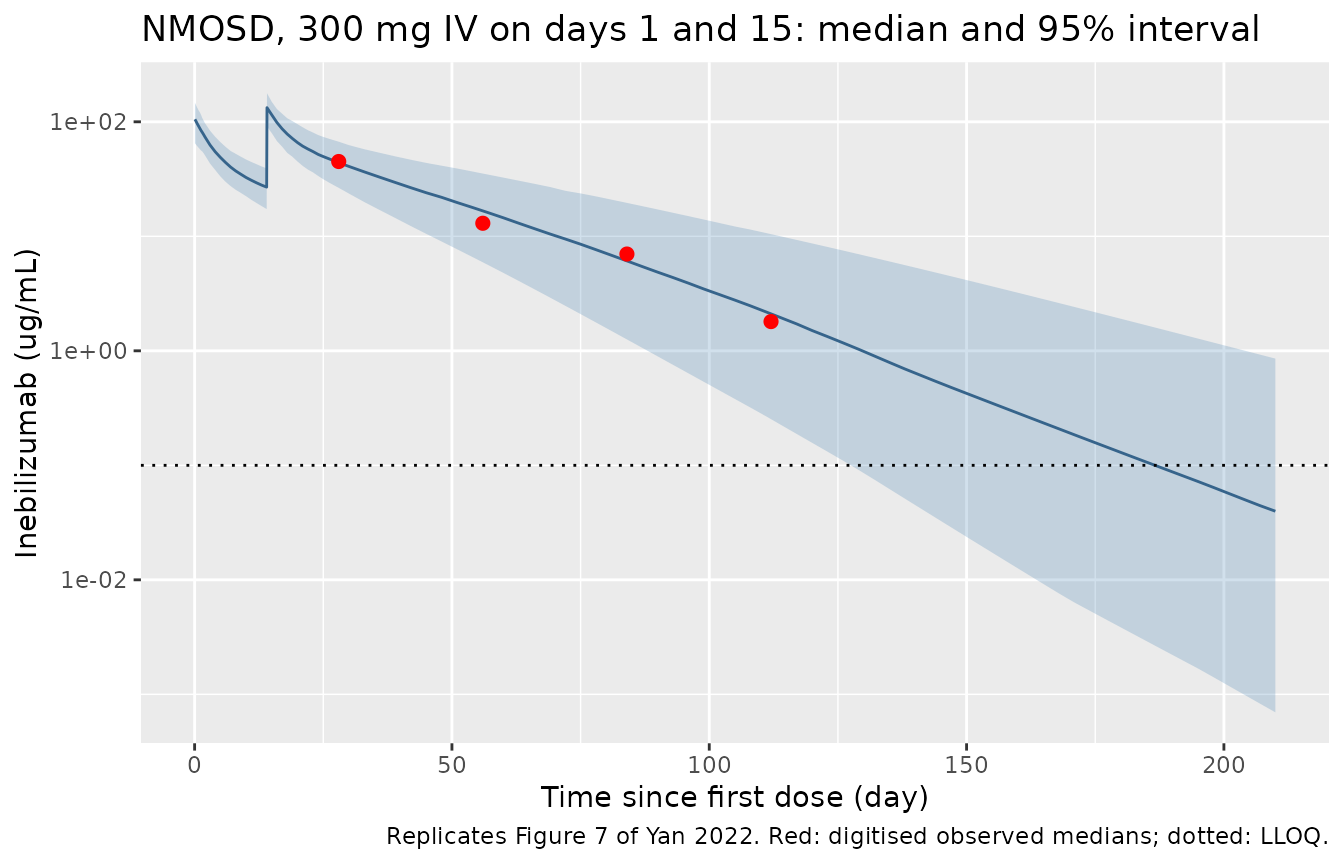
The typical-value (all random effects zero) profile at the median NMOSD weight is compared with the digitised medians below. It removes cohort noise from the check.
ev_typ <- rxode2::et(amt = 300, cmt = "central", dur = inf_dur) |>
  rxode2::et(time = 14, amt = 300, cmt = "central", dur = inf_dur) |>
  rxode2::et(fig7_digitised$time, cmt = "central") |>
  as.data.frame() |>
  mutate(WT = 65.0, STUDY_MICP200 = 0)

typ <- rxode2::rxSolve(mod_typ, events = ev_typ) |>
  as.data.frame() |>
  select(time, Cc)
#> ℹ omega/sigma items treated as zero: 'etalcl', 'etalvc', 'etalvp', 'etalvmax'

fig7_cmp <- fig7_digitised |>
  left_join(typ, by = "time") |>
  mutate(ratio = Cc / obs_median)

fig7_cmp |>
  rename(
    "Day" = time,
    "Digitised observed median (ug/mL)" = obs_median,
    "Typical-value model (ug/mL)" = Cc,
    "Model / observed" = ratio
  ) |>
knitr::kable(digits = 2)| Day | Digitised observed median (ug/mL) | Typical-value model (ug/mL) | Model / observed |
|---|---|---|---|
| 28 | 45.0 | 44.76 | 0.99 |
| 56 | 13.0 | 17.08 | 1.31 |
| 84 | 7.0 | 6.15 | 0.88 |
| 112 | 1.8 | 2.03 | 1.13 |
Dose nonlinearity in the SSc single-ascending-dose study
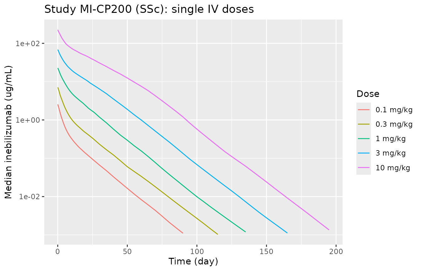
Yan 2022 notes that phase I NCA showed a more than dose-proportional rise in exposure. The model shows the same thing. As the dose falls toward Km, the saturable pathway takes a larger share of elimination, so dose-normalised AUC drops at low doses. The single-dose cohorts of study MI-CP200 (0.1-10 mg/kg) are simulated with the systemic-sclerosis study effect on Vmax.
ssc_doses <- c(0.1, 0.3, 1, 3, 10)
ssc_obs <- sort(unique(c(seq(0, 2, by = 0.25), inf_dur, seq(3, 28, by = 1), seq(30, 400, by = 5))))
events_ssc <- bind_rows(lapply(seq_along(ssc_doses), function(i) {
  make_cohort(
    50,
    dose_mgkg = ssc_doses[i], dose_times = 0, median_wt = 73.2,
    study_micp200 = 1, obs_times = ssc_obs,
    cohort = paste(ssc_doses[i], "mg/kg"), id_offset = (i - 1L) * 50L
  )
}))
stopifnot(!anyDuplicated(unique(events_ssc[, c("id", "time", "evid")])))

sim_ssc <- rxode2::rxSolve(mod, events = events_ssc, keep = c("cohort", "WT")) |>
  as.data.frame()
sim_ssc |>
  filter(time > 0) |>
  mutate(cohort = factor(cohort, levels = paste(ssc_doses, "mg/kg"))) |>
  group_by(cohort, time) |>
  summarise(Q50 = median(Cc), .groups = "drop") |>
  filter(Q50 > 1e-3) |>
  ggplot(aes(time, Q50, colour = cohort)) +
  geom_line() +
  scale_y_log10() +
  labs(
    x = "Time (day)", y = "Median inebilizumab (ug/mL)", colour = "Dose",
    title = "Study MI-CP200 (SSc): single IV doses"
  )
PKNCA validation
PKNCA is run on the SSc single-dose cohorts to measure dose-normalised exposure, and on the NMOSD cohort for the first 14-day dosing interval. Yan 2022 reports no NCA table, so no side-by-side published comparison is possible.
conc_ssc <- sim_ssc |>
  filter(!is.na(Cc)) |>
  select(id, time, Cc, cohort)
dose_ssc <- events_ssc |>
  filter(evid == 1) |>
  select(id, time, amt, cohort)

nca_ssc <- PKNCA::pk.nca(PKNCA::PKNCAdata(
  PKNCA::PKNCAconc(conc_ssc, Cc ~ time | cohort + id),
  PKNCA::PKNCAdose(dose_ssc, amt ~ time | cohort + id),
  intervals = data.frame(start = 0, end = Inf, cmax = TRUE, aucinf.obs = TRUE, half.life = TRUE)
))

ssc_tbl <- as.data.frame(nca_ssc$result) |>
  filter(PPTESTCD %in% c("cmax", "aucinf.obs", "half.life")) |>
  left_join(dose_ssc |> select(id, amt), by = "id") |>
  mutate(value = ifelse(PPTESTCD == "half.life", PPORRES, PPORRES / amt)) |>
  group_by(cohort, PPTESTCD) |>
  summarise(median = median(value, na.rm = TRUE), .groups = "drop") |>
  tidyr::pivot_wider(names_from = PPTESTCD, values_from = median) |>
  mutate(cohort = factor(cohort, levels = paste(ssc_doses, "mg/kg"))) |>
  arrange(cohort)

ssc_tbl |>
  rename(
    "Dose" = cohort,
    "Cmax / dose (ug/mL per mg)" = cmax,
    "AUCinf / dose (day*ug/mL per mg)" = aucinf.obs,
    "Terminal half-life (day)" = half.life
  ) |>
knitr::kable(digits = 3, caption = "Median simulated NCA by SSc dose cohort.")| Dose | AUCinf / dose (day*ug/mL per mg) | Cmax / dose (ug/mL per mg) | Terminal half-life (day) |
|---|---|---|---|
| 0.1 mg/kg | 1.788 | 0.335 | 14.873 |
| 0.3 mg/kg | 1.992 | 0.325 | 14.715 |
| 1 mg/kg | 2.405 | 0.319 | 14.377 |
| 3 mg/kg | 3.199 | 0.316 | 14.143 |
| 10 mg/kg | 3.901 | 0.308 | 13.642 |
The dose-normalised AUC should rise with dose and approach, without
reaching, the limit set by linear clearance alone as the saturable
pathway is swamped. For a 73.2 kg subject that limit is
1 / CL = 1 / (0.188 * (73.2/66.2)^0.57). The checks use the
typical subject, so there is no cohort noise.
typ_auc <- sapply(ssc_doses, function(d) {
  ev <- rxode2::et(amt = d * 73.2, cmt = "central", dur = inf_dur) |>
    rxode2::et(seq(0, 1500, by = 0.5), cmt = "central") |>
    as.data.frame() |>
    mutate(WT = 73.2, STUDY_MICP200 = 1)
  s <- as.data.frame(rxode2::rxSolve(mod_typ, events = ev))
  sum(diff(s$time) * (head(s$Cc, -1) + tail(s$Cc, -1)) / 2) / (d * 73.2)
})
#> ℹ omega/sigma items treated as zero: 'etalcl', 'etalvc', 'etalvp', 'etalvmax'
#> ℹ omega/sigma items treated as zero: 'etalcl', 'etalvc', 'etalvp', 'etalvmax'
#> ℹ omega/sigma items treated as zero: 'etalcl', 'etalvc', 'etalvp', 'etalvmax'
#> ℹ omega/sigma items treated as zero: 'etalcl', 'etalvc', 'etalvp', 'etalvmax'
#> ℹ omega/sigma items treated as zero: 'etalcl', 'etalvc', 'etalvp', 'etalvmax'
cl_lin <- exp(p[["lcl"]]) * (73.2 / 66.2)^p[["e_wt_cl"]]
data.frame(dose_mgkg = ssc_doses, auc_per_mg = typ_auc, linear_limit = 1 / cl_lin)
#>   dose_mgkg auc_per_mg linear_limit
#> 1       0.1   1.677043     5.022962
#> 2       0.3   1.907552     5.022962
#> 3       1.0   2.420307     5.022962
#> 4       3.0   3.131930     5.022962
#> 5      10.0   3.942096     5.022962

stopifnot(
  all(diff(typ_auc) > 0),
  typ_auc[5] < 1 / cl_lin,
  typ_auc[5] / typ_auc[1] > 1.5
)
conc_nmosd <- sim_nmosd |>
  filter(!is.na(Cc)) |>
  select(id, time, Cc, cohort)
dose_nmosd <- events_nmosd |>
  filter(evid == 1, time == 0) |>
  select(id, time, amt, cohort)

nca_nmosd <- PKNCA::pk.nca(PKNCA::PKNCAdata(
  PKNCA::PKNCAconc(conc_nmosd, Cc ~ time | cohort + id),
  PKNCA::PKNCAdose(dose_nmosd, amt ~ time | cohort + id),
  intervals = data.frame(start = 0, end = 14, cmax = TRUE, tmax = TRUE, auclast = TRUE)
))

nmosd_tbl <- as.data.frame(nca_nmosd$result) |>
  group_by(cohort, PPTESTCD) |>
  summarise(
    median = median(PPORRES, na.rm = TRUE),
    Q05 = quantile(PPORRES, 0.05, na.rm = TRUE),
    Q95 = quantile(PPORRES, 0.95, na.rm = TRUE),
    .groups = "drop"
  )
knitr::kable(nmosd_tbl, digits = 2, caption = "Simulated NCA over the first 14-day interval, NMOSD 300 mg.")| cohort | PPTESTCD | median | Q05 | Q95 |
|---|---|---|---|---|
| NMOSD 300 mg x2 | auclast | 666.23 | 488.01 | 860.59 |
| NMOSD 300 mg x2 | cmax | 105.20 | 72.33 | 140.00 |
| NMOSD 300 mg x2 | tmax | 0.06 | 0.06 | 0.06 |
# Linear-clearance upper bound on AUC0-14 of 300 mg is well above the simulated
# median; a 1000-fold unit slip in V or CL would push the median far outside
# this window. Centre-of-distribution checks only.
auc14 <- nmosd_tbl$median[nmosd_tbl$PPTESTCD == "auclast"]
cmax1 <- nmosd_tbl$median[nmosd_tbl$PPTESTCD == "cmax"]
stopifnot(
  auc14 > 300 / 0.188 / 10, auc14 < 300 / 0.188,
  cmax1 > 50, cmax1 < 300 / 2.95 * 1.5
)
Subcutaneous dosing
Six MS subjects in study 1102 received single SC doses of 60 or 300 mg. The paper reports only the resulting absorption half-life (4.1 days) and absolute bioavailability (81%). The plot shows typical-value profiles for the two SC doses next to the equivalent IV doses.
sc_ev <- function(dose, route, id) {
  obs <- data.frame(id = id, time = seq(0, 150, by = 0.5), amt = 0, evid = 0L,
                    cmt = "central", dur = 0)
  dose_row <- data.frame(id = id, time = 0, amt = dose, evid = 1L,
                         cmt = if (route == "SC") "depot" else "central",
                         dur = if (route == "SC") 0 else inf_dur)
  bind_rows(dose_row, obs) |>
    mutate(regimen = paste(dose, "mg", route))
}
ev_sc <- bind_rows(
  sc_ev(60, "SC", 1L), sc_ev(60, "IV", 2L),
  sc_ev(300, "SC", 3L), sc_ev(300, "IV", 4L)
) |>
  mutate(WT = 72.0, STUDY_MICP200 = 0)
sim_sc <- rxode2::rxSolve(mod_typ, events = ev_sc, keep = "regimen") |> as.data.frame()
#> ℹ omega/sigma items treated as zero: 'etalcl', 'etalvc', 'etalvp', 'etalvmax'
#> Warning: multi-subject simulation without without 'omega'

ggplot(filter(sim_sc, time > 0), aes(time, Cc, colour = regimen)) +
  geom_line() +
  scale_y_log10() +
  labs(x = "Time (day)", y = "Inebilizumab (ug/mL)", colour = NULL,
       title = "Typical-value SC vs IV profiles (72 kg MS subject)")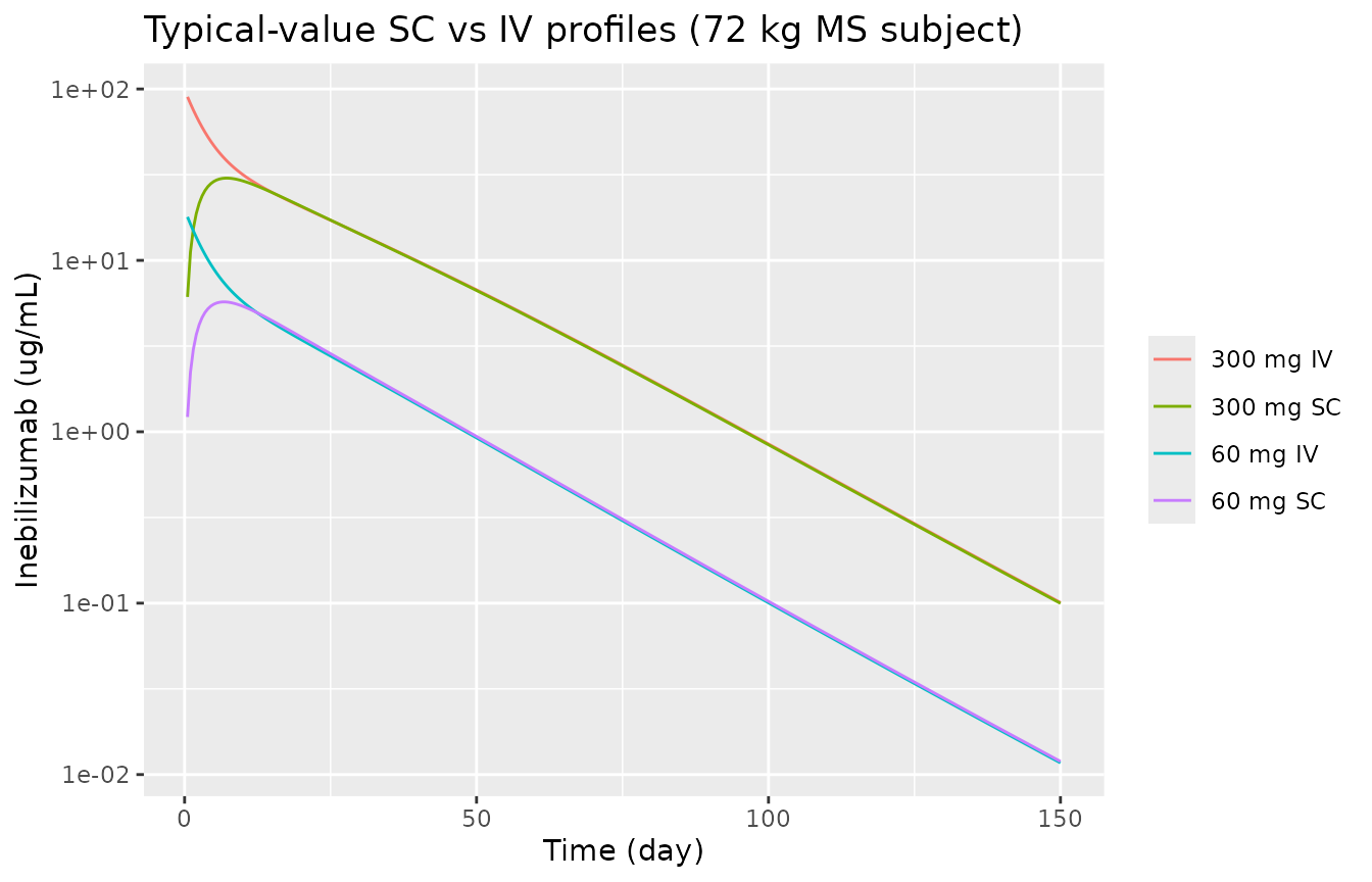
Assumptions and deviations
-
Study MI-CP200 effect on Vmax. Table 6 reports
‘Study CP200 on Vmax (%)’ = 210, and Eq. 4 defines categorical effects
as fractional changes,
P = theta1 * (1 + theta2 * Factor). The model therefore usesVmax * (1 + 2.10 * STUDY_MICP200), a 3.1-fold ratio. The Discussion says that Vmax in SSc subjects “was 2.1-fold higher”. The maintainers read this as a paraphrase of the 210% increase and kept the equation. If the phrase instead means a 2.1-fold ratio, the SSc Vmax would be about a third lower. This affects onlySTUDY_MICP200 = 1subjects. The FDA review lists the same estimate (209.91%) and does not settle the question. -
Study effect vs disease. All MI-CP200 subjects had
SSc, so the study indicator is confounded with disease. The model keeps
the paper’s study labelling (
STUDY_MICP200) rather than recasting it as a disease covariate. -
IIV scale. Table 6 gives IIV as %CV. The variances
are
log(CV^2 + 1): 27% becomes 0.0704 (CL), 17% becomes 0.0285 (Vc), 16% becomes 0.0253 (Vp) and 30% becomes 0.0862 (Vmax). The CL-Vmax covariance was not retained (Table 4, model 7). - Residual error. Section 2.5.4 describes a combined proportional and additive error model. The final model (Table 6, and the Section 3.3 statement that the proportional error model was sufficient) has a proportional term only, and the FDA review agrees, so no additive term is included.
-
Time origin for the Vmax decline. Eq. 8 uses NONMEM
time, taken here as time since the first dose. Simulations must start at the first dose. -
Subcutaneous parameters.
ka = log(2)/4.1 = 0.169 1/dayandF = 0.81come from the absorption half-life and bioavailability in Section 3.4. The paper does not say whether any IV parameter was re-estimated in the combined SC fit or whether the absorption parameters had IIV. The IV parameters of the final IV model (model 5) are used unchanged, with no IIV onkaorF. The authors warn that n = 6 is too small to estimate SC bioavailability reliably. - Infusion duration. Not reported in Yan 2022; 1.5 h is assumed for every IV dose. For an antibody with a half-life of weeks, this has no visible effect beyond the first hours.
- Half-life. The paper gives “approximately 18 days” at the therapeutic dose. The linear two-compartment beta half-life of the typical subject is about 23 days. Adding the residual Michaelis-Menten arm at the low concentrations reached after the second 300 mg dose brings the apparent half-life over days 150-250 close to 17-18 days. The 18-day figure is therefore not asserted.
- Figure numbering. The Results text calls Figure 6 the NMOSD VPC and Figure 7 the all-subject VPC, but the captions have them the other way round. This vignette follows the captions: Figure 7 is the NMOSD VPC.
- Virtual weights. Log-normal around each study’s median weight (NMOSD 65.0 kg, SSc 73.2 kg; Table 2), with sdlog 0.25. Values outside the observed 38-148 kg range are redrawn.
- Parameter precision. Values come from Table 6 of the article. The FDA review prints the same estimates to more digits (CL 188.22 mL/day, Vc 2946.39 mL, Q 363.23 mL/day, Vp 2569.43 mL, Vmax 832.50 ug/day, 209.91%, 21.78%); the article values are used.
- No erratum or correction notice for Yan 2022 was found (checked 2026-09-30).