Colistin sulfate (Yu 2022)
Source:vignettes/articles/Yu_2022_colistinSulfate.Rmd
Yu_2022_colistinSulfate.RmdModel and source
- Citation: Yu XB, Zhang XS, Wang YX, Wang YZ, Zhou HM, Xu FM, Yu JH, Zhang LW, Dai Y, Zhou ZY, Zhang CH, Lin GY, Pan JY (2022). Population pharmacokinetics of colistin sulfate in critically ill patients: exposure and clinical efficacy. Front Pharmacol 13:915958. doi:10.3389/fphar.2022.915958. See also the published commentary: Chen H, Li P (2022). Commentary: Population pharmacokinetics of colistin sulfate in critically ill patients: exposure and clinical efficacy. Front Pharmacol 13:992085. doi:10.3389/fphar.2022.992085.
- Description: One-compartment population PK model for intravenous colistin sulfate in critically ill adults with carbapenem-resistant organism infections (Yu 2022; n = 42 Chinese patients, 112 sparse steady-state therapeutic- drug-monitoring plasma concentrations spanning 0.28-6.20 mg/L). Linear elimination with intravenous-infusion input. Cockcroft-Gault creatinine clearance enters clearance as an additive linear term, CL = 0.994 + 0.525 * CrCL / 66.47 L/h, with exponential inter-individual variability on CL only and a proportional residual error. Colistin sulfate is the active drug and must not be confused with colistimethate sodium (CMS), the inactive prodrug modelled in Plachouras 2009, Mohamed 2012, Jacobs 2016 and Karaiskos 2015. Doses are in mg; the paper reports doses only in international units and its stated conversion is contradicted by its own simulations (see the vignette).
- Article: https://doi.org/10.3389/fphar.2022.915958
- Commentary: Chen H, Li P (2022), https://doi.org/10.3389/fphar.2022.992085
The final model is fully specified in the main text (Eqs. 1-2 and Table 3). The supplement holds the base model (Table S1), the bootstrap (Table S2) and the VPC (Figure S2); none of these is needed to reproduce the final model. No erratum has been published (Europe PMC search, 2026-10-02), but a published commentary by Chen and Li (2022) disputes the paper’s IU-to-mg conversion and its target-attainment reasoning. Both points are taken up below.
Colistin sulfate is the active polymyxin E salt,
given intravenously as such. It is not colistimethate sodium (CMS), the
inactive prodrug whose PK is modelled separately in this library by
Plachouras_2009_colistin,
Mohamed_2012_colistin, Jacobs_2016_colistin
and Karaiskos_2015_colistin. Other colistin sulfate models
in the library are Sun_2025_colistinSulfate,
Ma_2026_colistinSulfate,
Jin_2026_colistinSulfate and
Huang_2025_colistinSulfate.
Population
Forty-two critically ill adults (37 male, 5 female) treated with intravenous colistin sulfate for at least 3 days for confirmed carbapenem-resistant Gram-negative infections at the First Affiliated Hospital of Wenzhou Medical University between January 2020 and December 2021 (Methods, “Patients and Ethics”; Table 1). Age was 67.90 +/- 13.74 years, body weight 63.47 +/- 9.64 kg, serum creatinine 116.64 +/- 105.49 umol/L and Cockcroft-Gault creatinine clearance 79.54 +/- 53.99 mL/min (mean +/- SD). APACHE II was 17 [14, 26]; 76.19% were mechanically ventilated. The respiratory tract was the most common infection site (69.05%) and Acinetobacter baumannii the most common isolate (73.81%).
The label regimen is a 1 million IU loading dose followed by 1.5 million IU per day in 2-3 divided doses; the Table 1 daily dose was 150 [150, 200] x 10^4 IU. Twenty-two patients also received inhaled colistin sulfate and four received it intraventricularly or intrathecally. Steady-state sparse samples (after at least six doses) gave 112 plasma concentrations from 0.28 to 6.20 mg/L. Concentrations drawn during renal replacement therapy or ECMO were excluded.
The same information is available programmatically via
readModelDb("Yu_2022_colistinSulfate")()$population.
Source trace
| Equation / parameter | Value | Source location |
|---|---|---|
lcl (CL intercept, L/h) |
0.994 | Table 3 TVCL (L/h) 0.994 (RSE 16%); Eq. 1 |
e_crcl_cl (L/h per CrCL/66.47) |
0.525 | Table 3 CrCL on CL (theta 1) 0.525 (RSE 22%); Eq.
1 |
| CrCL divisor | 66.47 mL/min | Eq. 1 and Table 4 only; not tabulated as a cohort statistic |
lvc (V, L) |
20.7 | Table 3 TVV (L) 20.7 (RSE 10%); Eq. 2 |
etalcl |
omega^2 = 0.08835 | Table 3 BSV_CL [%CV] 30.40% (RSE 15%, shrinkage 9%);
log(0.304^2 + 1)
|
propSd |
0.251 | Table 3 Proportional error [%CV] 25.10% (RSE 16%,
shrinkage 14%) |
cl <- (exp(lcl) + e_crcl_cl * CRCL / 66.47) * exp(etalcl) |
n/a | Eq. 1; Methods “exponential function” for BSV |
vc <- exp(lvc) |
n/a | Eq. 2 (no covariate, no IIV in the final model) |
d/dt(central) <- -kel * central |
n/a | Results: “one-compartmental model with linear elimination” |
Cc ~ prop(propSd) |
n/a | Results: “The proportional error model was selected” |
mod <- readModelDb("Yu_2022_colistinSulfate")
ui <- rxode2::rxode(mod)
#> ℹ parameter labels from comments will be replaced by 'label()'
omega_cl <- sqrt(ui$omega["etalcl", "etalcl"])
cl_typ <- function(crcl) 0.994 + 0.525 * crcl / 66.47   # Eq. 1

# The packaged typical clearance must equal Eq. 1 exactly.
crcl_grid <- seq(10, 120, by = 10)
typ <- rxode2::rxSolve(
  rxode2::zeroRe(ui),
  events = data.frame(id = seq_along(crcl_grid), time = 0, evid = 0,
                      amt = 0, cmt = "central", CRCL = crcl_grid),
  keep = "CRCL"
) |> as.data.frame()
#> ℹ omega/sigma items treated as zero: 'etalcl'
#> Warning: multi-subject simulation without without 'omega'
stopifnot(max(abs(typ$cl / cl_typ(typ$CRCL) - 1)) < 1e-10)
The dose unit
The model works in mg and mg/L, as the paper’s parameters and assay do. The paper reports every dose in international units. Three candidate conversions are in play:
| Conversion | mg per 10^6 IU | Source |
|---|---|---|
| 17,000 IU per mg | 58.8 | Yu 2022 Introduction: “1 mg of pure colistin base = 17,000 IU of colistin” |
| about 22,300 IU per mg | 44.8 | Chinese consensus figure for colistin sulfate quoted by Chen and Li (2022), who show that 17,000 IU/mg is only the pharmacopoeial lower potency limit |
| 30,000 IU per mg | 33.3 | the colistin-base-activity convention |
The conversion used in the authors’ NONMEM dataset decides what “mg”
means for this model, and the paper’s own model-based output identifies
it. Figure 3 plots the probability of target attainment (PTA,
fAUC/MIC >= 15, unbound fraction 0.5) against creatinine
clearance for six regimens, each with a loading dose of twice the
maintenance dose (Methods, “Monte Carlo Simulations”).
Which AUC Figure 3 uses
Figure 3 cannot be a steady-state AUC. At steady state a linear model
gives AUC0-24 = daily dose / CL, so 750 KU q12h and 500 KU
q8h (both 1.5 MU/day) would have identical curves, as would 1 MU q12h
and 750 KU q8h (2.0 versus 2.25 MU/day, a fixed 12% apart). Instead
Figure 3 draws 750 KU q12h well above 500 KU q8h and 1 MU q12h on top of
750 KU q8h, and the Results say that “with the same daily dose, the
dosing interval of 12 h had higher PTA achievement than the dosing
interval of 8 h”. Chen and Li (2022) note that this “is not possible for
an AUC-based PK/PD index and a PK model with linear elimination” at
steady state. What the figure does fit is an AUC driven by the
first day’s doses including the loading dose: 750 KU
q12h delivers 1.5 + 0.75 = 2.25 MU in the first 24 h against 1.0 + 0.5 +
0.5 = 2.0 MU for 500 KU q8h, and 1 MU q12h and 750 KU q8h both deliver
3.0 MU. The total exposure from those doses is
AUC = D(first 24 h) / CL, which is log-normal in CL, so the
PTA at each creatinine clearance is a closed-form probability.
# Maintainer-digitised from Figure 3 of Yu 2022 (PTA, %, read off the fitted
# curves at CrCL 10, 40, 80 and 120 mL/min; roughly +/- 2 percentage points).
# Curves pinned at 100% (all of MIC = 0.5, and 750 KU q8h / 1 MU q12h /
# 1 MU q8h at MIC = 1) carry no information and are omitted.
fig3 <- tibble::tribble(
  ~MIC, ~regimen,     ~mu_maint, ~tau, ~c10, ~c40, ~c80, ~c120,
  1,    "500KU q12h", 0.50,      12,   90.5, 74,   48,   27,
  1,    "500KU q8h",  0.50,       8,   99,   95.5, 84,   64,
  1,    "750KU q12h", 0.75,      12,   99.5, 98,   90.5, 76,
  2,    "500KU q12h", 0.50,      12,   16,    5,    1,    0.3,
  2,    "500KU q8h",  0.50,       8,   52,   27,   10,    3,
  2,    "750KU q12h", 0.75,      12,   66,   40,   18,    6.5,
  2,    "750KU q8h",  0.75,       8,   92,   77,   51,   31,
  2,    "1MU q12h",   1.00,      12,   91,   76,   50,   28,
  2,    "1MU q8h",    1.00,       8,   99,   95,   83,   64.5
) |>
  pivot_longer(c10:c120, names_to = "crcl", values_to = "pta_pub",
               names_transform = list(crcl = function(x) as.numeric(sub("c", "", x)))) |>
  mutate(
    # MU given in the first 24 h: a 2x loading dose, then the maintenance
    # doses that fall before 24 h.
    mu_day1 = mu_maint * (2 + (24 / tau - 1)),
    # MU per day at steady state.
    mu_ss = mu_maint * 24 / tau
  )
stopifnot(nrow(fig3) == 36L)

pta_closed <- function(mu, mg_per_mu, crcl, mic) {
  # P(0.5 * mu * mg_per_mu / CL >= 15 * MIC) with CL = cl_typ * exp(eta)
  thr_cl <- 0.5 * mu * mg_per_mu / (15 * mic)
  100 * pnorm(log(thr_cl / cl_typ(crcl)) / omega_cl)
}

rmse_for <- function(mg_per_mu, which_mu) {
  pred <- pta_closed(fig3[[which_mu]], mg_per_mu, fig3$crcl, fig3$MIC)
  sqrt(mean((pred - fig3$pta_pub)^2))
}

fit_day1 <- optimize(rmse_for, c(15, 90), which_mu = "mu_day1")
fit_ss <- optimize(rmse_for, c(15, 90), which_mu = "mu_ss")
mg_per_mu <- fit_day1$minimum

scores <- tibble::tibble(
  `AUC definition` = c("First-24-h doses incl. loading / CL", "Steady-state daily dose / CL",
                       rep("First-24-h doses incl. loading / CL", 3)),
  `Conversion` = c("best fit", "best fit", "30,000 IU/mg (base activity)",
                   "22,300 IU/mg (consensus)", "17,000 IU/mg (as printed)"),
  `mg per 1e6 IU` = c(fit_day1$minimum, fit_ss$minimum, 1e6 / 30000,
                      1e6 / 22300, 1e6 / 17000)
) |>
  mutate(`RMSE vs Figure 3 (percentage points)` = c(
    fit_day1$objective, fit_ss$objective,
    vapply(`mg per 1e6 IU`[3:5], rmse_for, numeric(1), which_mu = "mu_day1")
  ))

knitr::kable(scores, digits = 2, caption = paste(
  "Figure 3 of Yu 2022 reproduced from the packaged model (typical CL from",
  "Eq. 1, omega from Table 3) under each candidate AUC definition and dose",
  "conversion. Closed-form probabilities, no simulated cohort."
))| AUC definition | Conversion | mg per 1e6 IU | RMSE vs Figure 3 (percentage points) |
|---|---|---|---|
| First-24-h doses incl. loading / CL | best fit | 32.48 | 1.07 |
| Steady-state daily dose / CL | best fit | 46.27 | 4.52 |
| First-24-h doses incl. loading / CL | 30,000 IU/mg (base activity) | 33.33 | 2.49 |
| First-24-h doses incl. loading / CL | 22,300 IU/mg (consensus) | 44.84 | 25.48 |
| First-24-h doses incl. loading / CL | 17,000 IU/mg (as printed) | 58.82 | 40.66 |
# Deterministic arithmetic on the packaged parameters and digitised points, so
# these bounds can be tight. The best-fit RMSE is about 1 percentage point,
# inside the digitisation error.
stopifnot(
  fit_day1$objective < 3,
  mg_per_mu > 30, mg_per_mu < 36,
  # The steady-state reading fits much worse at its own best conversion
  # (realised 4.5 vs 1.1 pp).
  fit_ss$objective > 3 * fit_day1$objective,
  # Neither printed nor consensus conversion reproduces the figure.
  scores$`RMSE vs Figure 3 (percentage points)`[4] > 10,
  scores$`RMSE vs Figure 3 (percentage points)`[5] > 10
)
The paper’s Figure 3 is reproduced to within 1.1 percentage points (RMSE over 36 digitised points) with 32.5 mg per million IU, the IIV of Table 3 and the first-24-h AUC. The recovered value is close to the colistin-base-activity convention (33.3 mg per million IU), and well away from both the 17,000 IU/mg printed in the paper (58.8 mg) and the 22,300 IU/mg consensus figure (44.8 mg), each of which misses the figure by tens of percentage points under the first-24-h AUC.
The steady-state reading deserves a fair hearing, because its own
best conversion (46.3 mg per million IU) is close to the consensus
figure. It fits 4.2 times worse (RMSE 4.5 against 1.1 percentage
points), and, more decisively, it forces regimens with the same daily
dose onto one curve, so it cannot produce the q12h-over-q8h separation
that both the figure and the Results text describe. The first-24-h
reading is therefore taken as the paper’s, and with it the milligram
scale of about 32.5 mg per million IU. The PTA depends on dose only
through mu * mg_per_mu / CL, so this establishes the
milligram scale on which the authors’ clearance is expressed, assuming
they simulated in the same units as they fitted. The Discussion’s
simulated “Cmin” and the Table 2 AUC (both below) are consistent with
it. The rest of this article converts IU regimens to mg with the
recovered value.
Replicating Figure 3
regs <- tibble::tribble(
  ~regimen,     ~mu_maint, ~tau,
  "500KU q12h", 0.50,      12,
  "500KU q8h",  0.50,       8,
  "750KU q12h", 0.75,      12,
  "750KU q8h",  0.75,       8,
  "1MU q12h",   1.00,      12,
  "1MU q8h",    1.00,       8
) |>
  mutate(mu_day1 = mu_maint * (2 + (24 / tau - 1)))

pta_grid <- crossing(regs, MIC = c(0.5, 1, 2), crcl = seq(10, 120, by = 5)) |>
  mutate(PTA = pta_closed(mu_day1, mg_per_mu, crcl, MIC))

ggplot(pta_grid, aes(crcl, PTA, colour = regimen)) +
  geom_line() +
  geom_point(data = fig3, aes(y = pta_pub), shape = 1) +
  geom_hline(yintercept = 90, linetype = "dashed") +
  facet_wrap(~ paste0("MIC = ", MIC, " mg/L")) +
  labs(x = "Creatinine clearance (mL/min)", y = "PTA (%)", colour = "Regimen",
       caption = paste("Replicates Figure 3 of Yu 2022. Lines: packaged model;",
                       "open points: digitised from the published figure.")) +
  theme(legend.position = "bottom")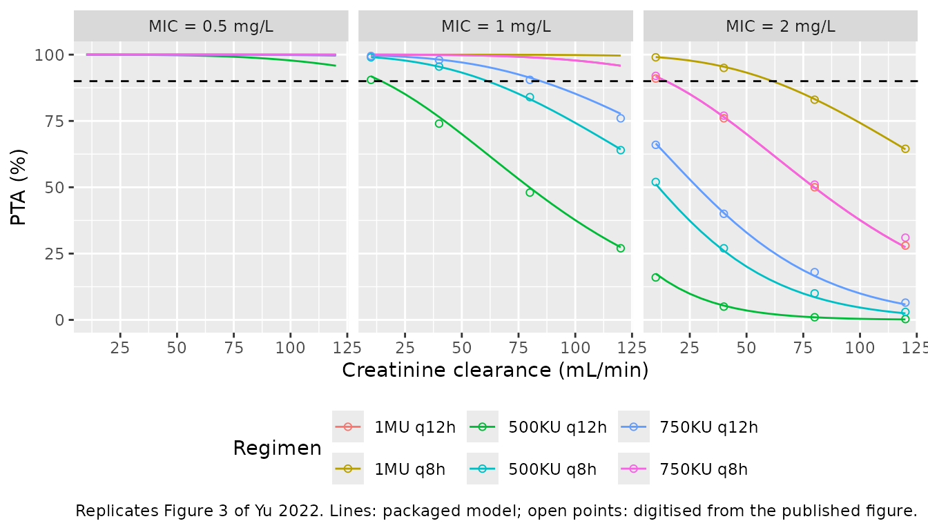
cell <- function(reg, mic, crcl) {
  v <- pta_grid$PTA[pta_grid$regimen == reg & pta_grid$MIC == mic & pta_grid$crcl == crcl]
  if (length(v) != 1L) stop("no unique PTA cell for '", reg, "'")
  v
}
pta_of <- function(regs_in, mic, crcl_in) {
  v <- pta_grid$PTA[pta_grid$regimen %in% regs_in & pta_grid$MIC == mic &
                      pta_grid$crcl %in% crcl_in]
  stopifnot(length(v) == length(regs_in) * length(crcl_in))
  v
}

claims <- tibble::tribble(
  ~Claim, ~Holds,
  "MIC 0.5: 500KU q12h, 500KU q8h and 750KU q12h exceed 90% at every CrCL",
  all(pta_of(c("500KU q12h", "500KU q8h", "750KU q12h"), 0.5, seq(10, 120, 5)) > 90),
  "MIC 1: 500KU q12h is subtherapeutic (below 90% above CrCL 20)",
  all(pta_of("500KU q12h", 1, seq(20, 120, 5)) < 90),
  "MIC 1: 750KU q12h falls below 90% at CrCL > 80",
  all(pta_of("750KU q12h", 1, seq(90, 120, 5)) < 90),
  "MIC 1: 1MU q12h and 750KU q8h exceed 90% at every CrCL",
  all(pta_of(c("1MU q12h", "750KU q8h"), 1, seq(10, 120, 5)) > 90),
  "Same daily dose: q12h beats q8h (750KU q12h vs 500KU q8h, MIC 2, CrCL 40)",
  cell("750KU q12h", 2, 40) > cell("500KU q8h", 2, 40) + 5
)

knitr::kable(claims, caption = paste(
  "Target-attainment statements in the Results of Yu 2022, checked against",
  "the packaged model with the recovered dose conversion."
))| Claim | Holds |
|---|---|
| MIC 0.5: 500KU q12h, 500KU q8h and 750KU q12h exceed 90% at every CrCL | TRUE |
| MIC 1: 500KU q12h is subtherapeutic (below 90% above CrCL 20) | TRUE |
| MIC 1: 750KU q12h falls below 90% at CrCL > 80 | TRUE |
| MIC 1: 1MU q12h and 750KU q8h exceed 90% at every CrCL | TRUE |
| Same daily dose: q12h beats q8h (750KU q12h vs 500KU q8h, MIC 2, CrCL 40) | TRUE |
# Deterministic closed-form probabilities.
stopifnot(nrow(claims) == 5L, all(claims$Holds))

# The Results also state that "all the simulated dose regimens could not
# achieve the PTA >= 90% for MIC >= 2". The published Figure 3 itself shows
# 1MU q8h above 90% at MIC 2 for CrCL up to about 60 mL/min, and the model
# reproduces the figure, not the sentence.
stopifnot(cell("1MU q8h", 2, 40) > 90, cell("1MU q8h", 2, 120) < 90)
All five checkable statements hold. One does not: the Results say no regimen reaches 90% at MIC >= 2 mg/L, but Figure 3 itself shows 1 MU q8h above 90% at MIC 2 for creatinine clearance below about 60 mL/min, and the model follows the figure (95% at 40 mL/min).
Virtual cohort
Original observed data are not publicly available. Creatinine clearance is drawn from a gamma distribution matched to the Table 1 mean and SD (79.54 +/- 53.99 mL/min); the shape of the distribution is not reported. Two arms follow the label regimen: a 1 million IU loading dose, then 1.5 million IU/day as either 750 KU q12h or 500 KU q8h, each by 1-hour infusion (the paper says only “intravenous drip”), for 14 days. Fourteen days is long enough for the slowest-clearing simulated subjects (half-life above 30 h) to reach steady state.
# set.seed() seeds R's RNG, not rxode2's simulation RNG, whose streams are
# partitioned per solver thread. Every cohort assertion below is written to
# hold for any cohort the model can produce.
set.seed(20221002)
n_arm <- 200

make_arm <- function(label, mu_maint, tau, id_offset) {
  subj <- tibble::tibble(
    id = id_offset + seq_len(n_arm),
    CRCL = rgamma(n_arm, shape = (79.54 / 53.99)^2, rate = 79.54 / 53.99^2),
    regimen = label
  )
  maint_times <- seq(tau, 336 - tau, by = tau)
  doses <- bind_rows(
    subj |> mutate(time = 0, amt = 1.0 * mg_per_mu),
    subj |> crossing(time = maint_times) |> mutate(amt = mu_maint * mg_per_mu)
  ) |>
    mutate(evid = 1L, rate = amt / 1, cmt = "central")
  obs <- subj |>
    crossing(time = sort(unique(c(seq(0, 24, by = 0.5), seq(312, 336, by = 0.25))))) |>
    mutate(evid = 0L, amt = NA_real_, rate = NA_real_, cmt = "central")
  bind_rows(doses, obs) |> arrange(id, time, desc(evid))
}

events <- bind_rows(
  make_arm("750KU q12h", 0.75, 12, 0L),
  make_arm("500KU q8h", 0.50, 8, n_arm)
)
stopifnot(length(unique(events$id)) == 2 * n_arm)
Simulation
sim <- rxode2::rxSolve(mod, events = events, keep = c("regimen", "CRCL")) |>
  as.data.frame()
#> ℹ parameter labels from comments will be replaced by 'label()'
stopifnot(all(c("Cc", "sim", "cl") %in% names(sim)), all(is.finite(sim$Cc)))
Individual clearance against the reported EBE summary
The Results report a mean +/- SD empirical Bayes CL of 1.74 +/- 0.61 L/h across the 42 patients (eta-shrinkage 9%, so the EBE spread is close to the true spread).
cl_subj <- sim |> distinct(id, regimen, CRCL, cl)
knitr::kable(tibble::tibble(
  Quantity = c("Mean CL (L/h)", "SD CL (L/h)"),
  Simulated = c(mean(cl_subj$cl), sd(cl_subj$cl)),
  `Yu 2022 (Results)` = c(1.74, 0.61)
), digits = 2)| Quantity | Simulated | Yu 2022 (Results) |
|---|---|---|
| Mean CL (L/h) | 1.69 | 1.74 |
| SD CL (L/h) | 0.65 | 0.61 |
Steady-state profile (Figure 1)
Figure 1 plots the 112 observed concentrations against time since the last dose. The simulated 750 KU q12h arm on day 14 is shown against the published observation range (0.28-6.20 mg/L).
ss <- sim |>
  filter(regimen == "750KU q12h", time >= 324) |>
  mutate(tad = time - 324) |>
  group_by(tad) |>
  summarise(Q05 = quantile(sim, 0.05), Q50 = median(Cc), Q95 = quantile(sim, 0.95),
            .groups = "drop")

ggplot(ss, aes(tad)) +
  geom_ribbon(aes(ymin = Q05, ymax = Q95), alpha = 0.2) +
  geom_line(aes(y = Q50)) +
  geom_hline(yintercept = c(0.28, 6.20), linetype = "dotted") +
  labs(x = "Time since last dose (h)", y = "Colistin concentration (mg/L)",
       caption = paste("Compare Figure 1 of Yu 2022. Line: median prediction;",
                       "ribbon: 5th-95th percentile with residual error;",
                       "dotted: published observed range."))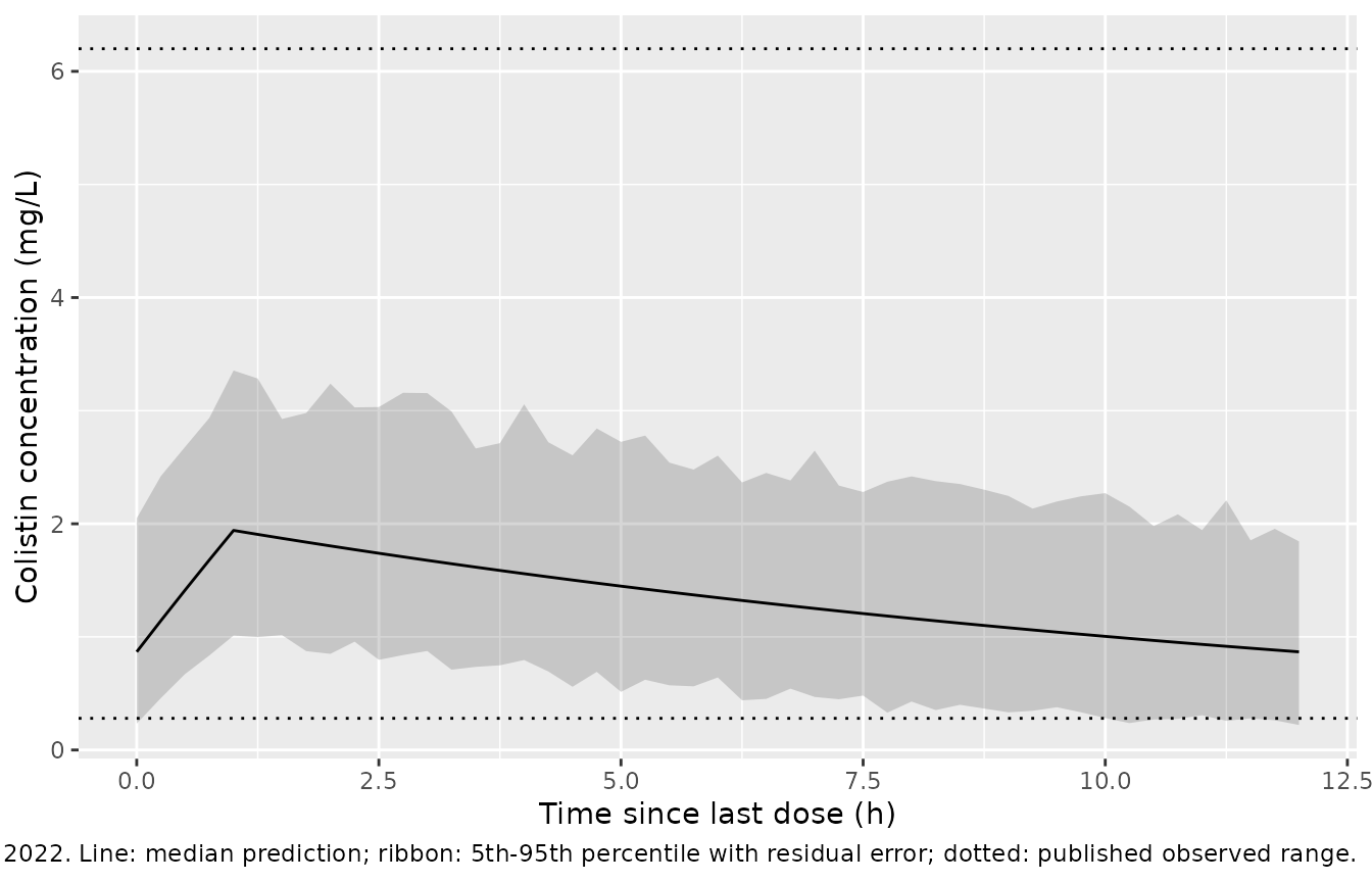
# Median profile sits inside the observed range at peak and trough.
stopifnot(
  ss$Q50[ss$tad == 1] > 0.28, ss$Q50[ss$tad == 1] < 6.20,
  ss$Q50[ss$tad == 12] > 0.28, ss$Q50[ss$tad == 12] < 6.20
)
PKNCA validation
sim_nca <- sim |>
  filter(!is.na(Cc)) |>
  mutate(Cc = pmax(Cc, 0)) |>
  select(id, time, Cc, regimen)

conc_obj <- PKNCA::PKNCAconc(sim_nca, Cc ~ time | regimen + id,
                             concu = "mg/L", timeu = "h")
dose_df <- events |> filter(evid == 1) |> select(id, time, amt, regimen)
dose_obj <- PKNCA::PKNCAdose(dose_df, amt ~ time | regimen + id, doseu = "mg")

tau_of <- c("750KU q12h" = 12, "500KU q8h" = 8)
intervals <- bind_rows(
  tibble::tibble(regimen = names(tau_of), start = 336 - tau_of, end = 336,
                 cmax = TRUE, cmin = TRUE, tmax = TRUE, auclast = TRUE),
  tibble::tibble(regimen = names(tau_of), start = 312, end = 336,
                 cmax = FALSE, cmin = FALSE, tmax = FALSE, auclast = TRUE)
) |> as.data.frame()

nca_res <- PKNCA::pk.nca(PKNCA::PKNCAdata(conc_obj, dose_obj, intervals = intervals))
nca_df <- as.data.frame(nca_res)
stopifnot(nrow(nca_df) > 0)
Closed-form identity
At steady state a one-compartment linear model gives
AUC0-tau = dose / CL exactly for the subject’s own drawn
clearance, so any difference is integration error.
auc_tau <- nca_df |>
  filter(PPTESTCD == "auclast", start > 312) |>
  select(id, regimen, auc = PPORRES) |>
  left_join(cl_subj, by = c("id", "regimen")) |>
  mutate(amt = unname(c("750KU q12h" = 0.75, "500KU q8h" = 0.50)[regimen]) * mg_per_mu,
         pct = 100 * (auc * cl / amt - 1))
stopifnot(nrow(auc_tau) == 2 * n_arm)

knitr::kable(tibble::tibble(
  Check = "AUC0-tau,ss vs dose / CL",
  `Median % difference` = median(auc_tau$pct),
  `Max abs % difference` = max(abs(auc_tau$pct))
), digits = 3)| Check | Median % difference | Max abs % difference |
|---|---|---|
| AUC0-tau,ss vs dose / CL | -0.003 | 0.073 |
Comparison against the published exposure
Table 2 and the Discussion report a MAP-estimated
AUC0-24,ss of 39.39 +/- 14.47 mg*h/L across the 42
patients. The study’s median daily dose was 1.5 million IU, which both
simulated arms deliver.
sim_auc24 <- nca_df |>
  filter(PPTESTCD == "auclast", start == 312) |>
  group_by(regimen) |>
  summarise(auclast = mean(PPORRES), .groups = "drop") |>
  as.data.frame()

published <- data.frame(regimen = names(tau_of), auclast = 39.39)

cmp <- nlmixr2lib::ncaComparisonTable(
  simulated = sim_auc24, reference = published, by = "regimen",
  units = c(auclast = "mg*h/L"), tolerance_pct = 20
)
knitr::kable(cmp, caption = paste(
  "Mean simulated AUC0-24,ss at 1.5 million IU/day against Yu 2022 Table 2.",
  "* differs from the reference by more than 20%."
), align = c("l", "l", "r", "r", "r"))| NCA parameter | regimen | Reference | Simulated | % diff |
|---|---|---|---|---|
| AUClast (mg*h/L) | 750KU q12h | 39.4 | 33.3 | -15.4% |
| AUClast (mg*h/L) | 500KU q8h | 39.4 | 33 | -16.2% |
# Cohort-derived; a mis-transcribed CL or a 44.8 / 58.8 mg-per-MU conversion
# moves this by 30-75%. The published patients' doses ranged up to 2 MU/day
# (Table 1 IQR 150-200 x 10^4 IU), so the simulated mean at the median dose is
# expected to sit somewhat low.
stopifnot(all(abs(sim_auc24$auclast / 39.39 - 1) < 0.30))
The simulated mean sits below the published value. That is expected: the simulation gives every subject the median 1.5 million IU/day, while a quarter of the study’s patients received 2 million IU/day or more (Table 1 interquartile range 150-200 x 10^4 IU). A dose conversion of 44.8 mg per million IU would raise the simulated value by 38%, and 58.8 mg by 81%.
The simulated “Cmin” of 1 MU q12h
The Discussion reports that the Cmin of 1 MU q12h “in simulated virtual patients was 2.33 +/- 1.13” mg/L, in the context of patients with creatinine clearance above 80 mL/min. The paper does not describe that simulation further.
ev_1mu <- tibble::tibble(id = 1:200, CRCL = seq(80, 150, length.out = 200)) |>
  crossing(time = seq(0, 156, by = 12)) |>
  mutate(evid = 1L, amt = ifelse(time == 0, 2, 1) * mg_per_mu, rate = amt,
         cmt = "central") |>
  bind_rows(tibble::tibble(id = 1:200, CRCL = seq(80, 150, length.out = 200)) |>
              crossing(time = c(157, 168)) |>
              mutate(evid = 0L, amt = NA_real_, rate = NA_real_, cmt = "central")) |>
  arrange(id, time, desc(evid))
s1 <- rxode2::rxSolve(mod, events = ev_1mu, keep = "CRCL") |> as.data.frame()

knitr::kable(tibble::tibble(
  Quantity = c("Cmax,ss (1 h)", "Cmin,ss (12 h)", "Yu 2022 'Cmin'"),
  `Mean (mg/L)` = c(mean(s1$Cc[s1$time == 157]), mean(s1$Cc[s1$time == 168]), 2.33),
  `SD (mg/L)` = c(sd(s1$Cc[s1$time == 157]), sd(s1$Cc[s1$time == 168]), 1.13)
), digits = 2)| Quantity | Mean (mg/L) | SD (mg/L) |
|---|---|---|
| Cmax,ss (1 h) | 2.33 | 0.47 |
| Cmin,ss (12 h) | 0.90 | 0.46 |
| Yu 2022 ‘Cmin’ | 2.33 | 1.13 |
cmax_ss <- mean(s1$Cc[s1$time == 157])
# Cohort mean of 200 subjects (SE about 2%). A 44.8 mg-per-MU conversion would
# put it 38% higher, a 58.8 conversion 81% higher.
stopifnot(abs(cmax_ss / 2.33 - 1) < 0.15)
The published mean of 2.33 mg/L matches the simulated peak (2.33 mg/L) under the recovered conversion, not the trough. No conversion among the three candidates brings the trough up to 2.33 mg/L (it would need roughly 80 mg per million IU), so the paper’s “Cmin” is most likely a mislabelled peak. Read that way, it is a second, independent confirmation of the recovered dose conversion: 44.8 mg per million IU would put the peak 38% higher. The published SD (1.13 mg/L) is wider than the simulated one, which the paper does not explain; its virtual-patient creatinine clearance distribution is not described.
Assumptions and deviations
- Dose conversion is derived, not printed. The paper states 17,000 IU per mg, and the commentary by Chen and Li (2022) states 22,300 IU per mg. Neither reproduces the paper’s own Figure 3. The conversion used throughout this article, 32.5 mg per million IU, is recovered from Figure 3 with the packaged model. The Discussion’s simulated 1 MU q12h concentration (read as a peak) and Table 2’s MAP AUC are consistent with it. The model itself takes doses in mg, so this only matters when restating IU regimens, but it does mean that a user who converts IU doses at 22,300 IU/mg (44.8 mg per million IU) will predict about 38% more exposure than the authors’ model implies.
- Figure 3 uses the first day’s doses. The regimen ordering in Figure 3 is reproduced only by an AUC equal to the total of the first 24 h of doses, including the loading dose, divided by CL. This is not a steady-state AUC, despite the clinical framing. Chen and Li (2022) made the same observation.
- Figure 3 values are digitised. The 36 PTA values were read off the published figure by the maintainers, to roughly +/- 2 percentage points.
-
IIV scale. Table 3 gives BSV on CL as 30.40 %CV; it
is converted with
omega^2 = log(CV^2 + 1) = 0.08835. Reading it asomega = 0.304instead (omega^2 = 0.0924) changes Figure 3 by under 0.2 percentage points RMSE, so the figure cannot separate the two readings. - CrCL divisor. 66.47 mL/min appears only in Eq. 1 and Table 4; it is not the reported mean (79.54 mL/min) and no median is reported.
- Non-intravenous routes are not modelled. 52% of patients also received inhaled colistin sulfate and 10% intraventricular or intrathecal doses, and the model treats only the intravenous drip as input. As Chen and Li (2022) note, any systemic absorption from those routes was attributed to the intravenous doses during fitting.
- Infusion duration. “Intravenous drip” is not quantified; 1-hour infusions are assumed. The PTA analysis does not depend on it.
- Creatinine clearance distribution. A gamma distribution matched to the Table 1 mean and SD; the true shape is unknown.
- Base model and BSV on V. BSV on V was estimated in the base model (Supplementary Table S1) but is absent from the final-model table, so the final model carries no IIV on V.
-
No PD model. The
fAUC/MIC >= 15target and unbound fraction 0.5 come from Cheah et al. (2015). The clinical efficacy and nephrotoxicity outcomes are descriptive; no exposure-response model was fitted.