Remdesivir (Roberts 2025)
Source:vignettes/articles/Roberts_2025_remdesivir.Rmd
Roberts_2025_remdesivir.RmdModel and source
- Citation: Roberts DM, Liu X, Parker SL, Burke A, Peek J, Carland JE, Murnion B, Seah V, Wallis SC, Sumi CD, Pandey S, Buscher H, Byrne A, Sandaradura I, Bowen D, Holz S, Stewart AG, Hajkowicz KM, Roberts JA. Population Pharmacokinetic Modelling of Remdesivir and Its Metabolite GS-441524 in Hospitalised Patients with COVID-19. Clin Pharmacokinet. 2025;64(5):743-756. doi:10.1007/s40262-025-01496-2.
- Description: Joint parent-metabolite population PK model for intravenous remdesivir and its circulating nucleoside metabolite GS-441524 in hospitalised adults with COVID-19 (Roberts 2025). Each compound is described by a one-compartment model with first-order elimination, coupled in series, so the system as a whole is the two-compartment model the paper describes (‘one compartment for each compound’). The entire model is written in molar units: the source converted both analytes from ng/mL to uM before fitting so that the parent-to-metabolite flux carries 1:1 stoichiometry despite the molecular-weight difference (remdesivir 602.585 g/mol, GS-441524 291.26 g/mol). Ten percent of remdesivir clearance was fixed to renal excretion of unchanged drug, so the remaining 90% (fm) is the flux that forms GS-441524. The fraction of that flux which actually appears as measurable plasma GS-441524 is not identifiable from plasma data alone, so the metabolite clearance and volume are apparent parameters (source CL/fm and V/fm) and the metabolite state carries an apparent amount; metabolite concentrations are nevertheless predicted correctly because the apparent volume and the apparent amount are scaled by the same unknown factor. Retained covariates are eGFR on GS-441524 clearance (power, exponent 1.12, reference 80 mL/min/1.73 m^2) and age on GS-441524 volume (power, exponent -1.15, reference 68.5 years); no covariate was retained on either remdesivir parameter. Between-subject variability was estimated on the clearance and volume of both compounds. Residual error is combined proportional-plus-additive for remdesivir and proportional for GS-441524.
- Article: https://doi.org/10.1007/s40262-025-01496-2
- Supplementary material (contains the MLXTRAN model listing used to verify the ODE structure, and Tables S1-S3): https://doi.org/10.1007/s40262-025-01496-2
Remdesivir is an intravenous monophosphoramidate prodrug. It is bioconverted in plasma through the alanine intermediate GS-704277 to the nucleoside metabolite GS-441524, which enters cells and is anabolised to the pharmacologically active triphosphate GS-443902. GS-441524 is the species actually quantified in plasma and, because it clears roughly seven-fold more slowly than the parent, it dominates systemic exposure. Roberts 2025 fitted both analytes simultaneously in one Monolix run.
Population
The model was built from a prospective, open-label, multi-centre, observational study in four Australian hospitals between July 2021 and August 2022 (Roberts 2025 Methods 2.1). Thirty-three adults hospitalised with nucleic-acid-test-confirmed SARS-CoV-2 infection and prescribed remdesivir were enrolled: median age 70 years (IQR 60-77, range 25-97), median baseline eGFR 80 mL/min/1.73 m^2 (range 33-124), and 21/33 (64%) male. Patients with eGFR < 30 mL/min/1.73 m^2 were excluded, so the model carries no information below that value.
Patients were split about 3:1 into model-building (n = 25) and external validation (n = 8) sets, with complete profiles prioritised for model building (Roberts 2025 Methods 2.3). The model-building set contributed 49 remdesivir concentrations from 12 patients and 153 GS-441524 concentrations from 25 patients; its median age was 69 years (IQR 60-73), median weight 92 kg (IQR 65-104, range 44-132) and median eGFR 72 mL/min/1.73 m^2 (IQR 59-87, range 34-124). Baseline characteristics are in Roberts 2025 Table 1. Every patient received the licensed regimen: remdesivir 200 mg intravenously on day 1 followed by 100 mg once daily from day 2 up to day 5 or day 10, each as a 60-minute infusion.
The same information is available programmatically via the model’s
population metadata
(readModelDb("Roberts_2025_remdesivir")()$population).
Source trace
The per-parameter origin is recorded as an in-file comment next to
each ini() entry in
inst/modeldb/specificDrugs/Roberts_2025_remdesivir.R. The
table below collects them in one place for review.
| Equation / parameter | Value | Source location |
|---|---|---|
lcl (remdesivir CL) |
105 L/h | Table 2, “Remdesivir CL” |
lvc (remdesivir V) |
121 L | Table 2, “Remdesivir V” |
fm (metabolic fraction of remdesivir CL) |
0.9, fixed | Methods 2.3 (“renal clearance of remdesivir was fixed to 10% of the
total remdesivir clearance”); Supplementary MLXTRAN listing
CLr = 0.1*CL, CLtr = 0.9*CL
|
lcl_gs441524 (GS-441524 CL/fm) |
15.9 L/h | Table 2, “GS-441524 CL/fm”; reference eGFR 80 from the Results 3.2 equation |
lvc_gs441524 (GS-441524 V/fm) |
429 L | Table 2, “GS-441524 V/fm”; reference age 68.5 y from the Results 3.2 equation |
e_crcl_cl_gs441524 |
1.12 | Table 2, “eGFR effect on CL”; Results 3.2 equation
(Cl/fm)_i = 15.9 * (eGFR_i/80)^1.12
|
e_age_vc_gs441524 |
-1.15 | Table 2, “Age effect on V”; Results 3.2 equation
(V/fm)_i = 429 * (Age_i/68.5)^-1.15
|
etalcl |
53.1% CV -> 0.24839 | Table 2, “Between subject variability (%) / Remdesivir CL” |
etalvc |
61.4% CV -> 0.31990 | Table 2, “Between subject variability (%) / Remdesivir V” |
etalcl_gs441524 |
36.8% CV -> 0.12701 | Table 2, “Between subject variability (%) / GS-441524 CL/fm” |
etalvc_gs441524 |
46.0% CV -> 0.19194 | Table 2, “Between subject variability (%) / GS-441524 V/fm” |
addSd |
0.014 uM | Table 2, “Remdesivir additive residual” |
propSd |
0.62 | Table 2, “Remdesivir proportional error” |
propSd_gs441524 |
0.16 | Table 2, “GS-441524 proportional error” |
d/dt(central) |
n/a | Supplementary MLXTRAN listing:
ddt_A1 = -(k10+k12)*A1
|
d/dt(central_gs441524) |
n/a | Supplementary MLXTRAN listing:
ddt_A2 = k12*A1 - k20*A2
|
Cc, Cc_gs441524
|
n/a | Supplementary MLXTRAN listing: C1 = A1/V1,
C2 = A2/V2
|
| Molar working units | MW 602.585 / 291.26 | Methods 2.3 (“concentration data were converted from ng/mL to uM”) |
The structural equations were verified line by line against the MLXTRAN model listing printed at the end of the Supplementary Material, which is reproduced here for reference:
CLr  = 0.1*CL              ; renal clearance of remdesivir
k10  = CLr/V1              ; rate constant of renal elimination of remdesivir
CLtr = 0.9*CL              ; metabolism clearance of remdesivir
k12  = CLtr/V1             ; remdesivir transformation rate constant to GS-441524
CLmi = CLm*(eGFR/80)^beta  ; covariate effects of eGFR on clearance of GS-441524
k20  = CLmi/V2             ; elimination rate constant of GS-441524
ddt_A1 = -(k10+k12)*A1     ; central compartment of remdesivir
ddt_A2 = k12*A1 - k20*A2   ; central compartment of GS-441524
C1 = A1/V1                 ; plasma concentration of remdesivir
C2 = A2/V2                 ; plasma concentration of GS-441524
Model structure
mod <- readModelDb("Roberts_2025_remdesivir")
ui <- rxode2::rxode2(mod)
#> ℹ parameter labels from comments will be replaced by 'label()'
ui
#>  ── rxode2-based free-form 2-cmt ODE model ──────────────────────────────────────
#>  ── Initalization: ──
#> Fixed Effects ($theta):
#>                lcl                lvc                 fm       lcl_gs441524
#>           4.653960           4.795791           0.900000           2.766319
#>       lvc_gs441524 e_crcl_cl_gs441524  e_age_vc_gs441524              addSd
#>           6.061457           1.120000          -1.150000           0.014000
#>             propSd    propSd_gs441524
#>           0.620000           0.160000
#>
#> Omega ($omega):
#>                  etalcl etalvc etalcl_gs441524 etalvc_gs441524
#> etalcl          0.24839 0.0000         0.00000         0.00000
#> etalvc          0.00000 0.3199         0.00000         0.00000
#> etalcl_gs441524 0.00000 0.0000         0.12701         0.00000
#> etalvc_gs441524 0.00000 0.0000         0.00000         0.19194
#> attr(,"lotriLabels")
#> [1] "Roberts 2025 Table 2: BSV remdesivir CL = 53.1% CV (RSE 29.5%, shrinkage 10.0%) -> omega^2 = log(1 + 0.531^2)"
#> [2] "Roberts 2025 Table 2: BSV remdesivir V = 61.4% CV (RSE 31.2%, shrinkage 12.8%) -> omega^2 = log(1 + 0.614^2)"
#> [3] "Roberts 2025 Table 2: BSV GS-441524 CL/fm = 36.8% CV (RSE 17.7%, shrinkage 6.91%) -> omega^2 = log(1 + 0.368^2)"
#> [4] "Roberts 2025 Table 2: BSV GS-441524 V/fm = 46.0% CV (RSE 22.1%, shrinkage -5.52%) -> omega^2 = log(1 + 0.460^2)"
#> attr(,"lotriFix")
#>                 etalcl etalvc etalcl_gs441524 etalvc_gs441524
#> etalcl           FALSE  FALSE           FALSE           FALSE
#> etalvc           FALSE  FALSE           FALSE           FALSE
#> etalcl_gs441524  FALSE  FALSE           FALSE           FALSE
#> etalvc_gs441524  FALSE  FALSE           FALSE           FALSE
#>
#> States ($state or $stateDf):
#>   Compartment Number Compartment Name
#> 1                  1          central
#> 2                  2 central_gs441524
#>  ── Multiple Endpoint Model ($multipleEndpoint): ──
#>          variable                        cmt                        dvid*
#> 1          Cc ~ …          cmt='Cc' or cmt=3          dvid='Cc' or dvid=1
#> 2 Cc_gs441524 ~ … cmt='Cc_gs441524' or cmt=4 dvid='Cc_gs441524' or dvid=2
#>   * If dvids are outside this range, all dvids are re-numered sequentially, ie 1,7, 10 becomes 1,2,3 etc
#>
#>  ── μ-referencing ($muRefTable): ──
#>          theta             eta level
#> 1          lcl          etalcl    id
#> 2          lvc          etalvc    id
#> 3 lcl_gs441524 etalcl_gs441524    id
#> 4 lvc_gs441524 etalvc_gs441524    id
#>
#>  ── Model (Normalized Syntax): ──
#> function() {
#>     compartmentData <- list(central = list(analyte = "remdesivir",
#>         units = "umol", specimen = "plasma", verified = TRUE),
#>         central_gs441524 = list(analyte = "GS-441524", units = "umol",
#>             specimen = "plasma", verified = TRUE))
#>     covariateData <- list(CRCL = list(description = "Estimated glomerular filtration rate calculated from serum creatinine with the CKD-EPI equation, BSA-normalised.",
#>         units = "mL/min/1.73 m^2", type = "continuous", reference_category = NULL,
#>         notes = "Roberts 2025 Methods 2.1: 'Estimated glomerular filtration rate (eGFR) was calculated on the basis of serum creatinine concentrations using the chronic kidney disease epidemiology collaboration formula (CKD-EPI) formula', with caution applied in patients with significant acute kidney injury. Patients with eGFR < 30 mL/min/1.73 m^2 were excluded, so the model is not informed below that value. Enters as a power effect on GS-441524 apparent clearance only, normalised to 80 mL/min/1.73 m^2 (the whole-cohort median): (CL/fm)_i = 15.9 * (eGFR_i / 80)^1.12. Baseline (not time-varying) eGFR was used.",
#>         source_name = "eGFR"), AGE = list(description = "Age at enrolment.",
#>         units = "years", type = "continuous", reference_category = NULL,
#>         notes = "Roberts 2025 Results 3.2 covariate equation: (V/fm)_i = 429 * (Age_i / 68.5)^-1.15. Note the normalising constant is 68.5 years, which is NOT the median age quoted elsewhere in the paper (70 years for the whole cohort, 69 years for the model-building subset); 68.5 is the value printed in the covariate equation and is what reproduces the reported typical volume, so it is used here verbatim. Cohort age range 25-97 years.",
#>         source_name = "Age"))
#>     description <- "Joint parent-metabolite population PK model for intravenous remdesivir and its circulating nucleoside metabolite GS-441524 in hospitalised adults with COVID-19 (Roberts 2025). Each compound is described by a one-compartment model with first-order elimination, coupled in series, so the system as a whole is the two-compartment model the paper describes ('one compartment for each compound'). The entire model is written in molar units: the source converted both analytes from ng/mL to uM before fitting so that the parent-to-metabolite flux carries 1:1 stoichiometry despite the molecular-weight difference (remdesivir 602.585 g/mol, GS-441524 291.26 g/mol). Ten percent of remdesivir clearance was fixed to renal excretion of unchanged drug, so the remaining 90% (fm) is the flux that forms GS-441524. The fraction of that flux which actually appears as measurable plasma GS-441524 is not identifiable from plasma data alone, so the metabolite clearance and volume are apparent parameters (source CL/fm and V/fm) and the metabolite state carries an apparent amount; metabolite concentrations are nevertheless predicted correctly because the apparent volume and the apparent amount are scaled by the same unknown factor. Retained covariates are eGFR on GS-441524 clearance (power, exponent 1.12, reference 80 mL/min/1.73 m^2) and age on GS-441524 volume (power, exponent -1.15, reference 68.5 years); no covariate was retained on either remdesivir parameter. Between-subject variability was estimated on the clearance and volume of both compounds. Residual error is combined proportional-plus-additive for remdesivir and proportional for GS-441524."
#>     population <- list(species = "human", n_subjects = 33L, n_studies = 1L,
#>         n_observations = "Model-building dataset: 49 remdesivir plasma concentrations from 12 patients and 153 GS-441524 plasma concentrations from 25 patients (Roberts 2025 Results 3.2). The 8 remaining patients formed an external-validation set used only to assess predictive performance (GS-441524 concentrations only).",
#>         age_range = "25-97 years (whole cohort; median 70, IQR 60-77). Model-building subset median 69 years (IQR 60-73; range 25-97); external-validation subset median 78 years (IQR 64-80; range 25-86).",
#>         age_median = "70 years", weight_range = "44-132 kg (model-building subset; median 92 kg, IQR 65-104). Weight was not recorded for the external-validation subset.",
#>         weight_median = "92 kg", sex_female_pct = 36.4, disease_state = "Adults (>18 years) admitted to hospital with SARS-CoV-2 infection confirmed by nucleic acid amplification test within 14 days of symptom onset, prescribed remdesivir for treatment of COVID-19. Worst disease severity in model-building survivors: mild 20%, moderate 16%, severe 40%, critical 20%. 72% received oxygen therapy, 30% were admitted to intensive care and 12% received ventilatory support. No patient had pre-existing chronic liver disease or received kidney replacement or vasopressor therapy.",
#>         renal_function = "Median baseline eGFR 80 mL/min/1.73 m^2 (range 33-124) in the whole cohort; model-building subset median 72 (IQR 59-87; range 34-124). Chronic kidney disease (eGFR 30-60) in 40% of the model-building subset. Patients with eGFR < 30 mL/min/1.73 m^2 were excluded from the study, so the model is uninformed below that value.",
#>         co_medication = "Corticosteroids (mostly dexamethasone) 88%, baricitinib 48%, tocilizumab 8%, sotrovimab 8%, antibiotics 24% (model-building subset; Table 1).",
#>         dose_range = "Licensed regimen only: remdesivir 200 mg intravenously on day 1 followed by 100 mg once daily from day 2 up to day 5 or day 10, each administered as a 60-minute infusion. No alternative regimen was studied clinically; the alternative regimens explored in the paper are simulation only.",
#>         regions = "Four hospitals in Australia (St Vincent's Hospital Sydney, The University of Queensland, Royal Brisbane and Women's Hospital and one further site), July 2021 to August 2022.",
#>         notes = "Prospective, open-label, multi-centre, observational study. Covariates tested but not retained: gender, height, body weight, BMI, SOFA score, serum albumin, bilirubin, ALT, AST, ALP and GGT (Roberts 2025 Methods 2.4). Baseline demographics are in Roberts 2025 Table 1. Estimation was by SAEM in Monolix 2021R2; the final model was checked by a 1000-run bootstrap (Rsmlx 4.0.2) and externally validated against the held-out 8 patients (median prediction error -15.2%, mean -19.5%, RMSE 30.5%).")
#>     reference <- "Roberts DM, Liu X, Parker SL, Burke A, Peek J, Carland JE, Murnion B, Seah V, Wallis SC, Sumi CD, Pandey S, Buscher H, Byrne A, Sandaradura I, Bowen D, Holz S, Stewart AG, Hajkowicz KM, Roberts JA. Population Pharmacokinetic Modelling of Remdesivir and Its Metabolite GS-441524 in Hospitalised Patients with COVID-19. Clin Pharmacokinet. 2025;64(5):743-756. doi:10.1007/s40262-025-01496-2."
#>     units <- list(time = "h", dosing = "umol", concentration = "umol/L")
#>     vignette <- "Roberts_2025_remdesivir"
#>     ini({
#>         lcl <- 4.65396035015752
#>         label("Remdesivir clearance CL (L/h)")
#>         lvc <- 4.79579054559674
#>         label("Remdesivir central volume of distribution V (L)")
#>         fm <- fix(0.9)
#>         label("Fraction of remdesivir clearance forming GS-441524 (unitless)")
#>         lcl_gs441524 <- 2.76631910922619
#>         label("GS-441524 apparent clearance CL/fm (L/h) at eGFR 80 mL/min/1.73 m^2")
#>         lvc_gs441524 <- 6.06145691892802
#>         label("GS-441524 apparent volume of distribution V/fm (L) at age 68.5 years")
#>         e_crcl_cl_gs441524 <- 1.12
#>         label("Power exponent for eGFR on GS-441524 apparent clearance (unitless)")
#>         e_age_vc_gs441524 <- -1.15
#>         label("Power exponent for age on GS-441524 apparent volume (unitless)")
#>         addSd <- c(0, 0.014)
#>         label("Remdesivir additive residual SD (uM)")
#>         propSd <- c(0, 0.62)
#>         label("Remdesivir proportional residual SD (fraction)")
#>         propSd_gs441524 <- c(0, 0.16)
#>         label("GS-441524 proportional residual SD (fraction)")
#>         etalcl ~ 0.24839
#>         label("Roberts 2025 Table 2: BSV remdesivir CL = 53.1% CV (RSE 29.5%, shrinkage 10.0%) -> omega^2 = log(1 + 0.531^2)")
#>         etalvc ~ 0.3199
#>         label("Roberts 2025 Table 2: BSV remdesivir V = 61.4% CV (RSE 31.2%, shrinkage 12.8%) -> omega^2 = log(1 + 0.614^2)")
#>         etalcl_gs441524 ~ 0.12701
#>         label("Roberts 2025 Table 2: BSV GS-441524 CL/fm = 36.8% CV (RSE 17.7%, shrinkage 6.91%) -> omega^2 = log(1 + 0.368^2)")
#>         etalvc_gs441524 ~ 0.19194
#>         label("Roberts 2025 Table 2: BSV GS-441524 V/fm = 46.0% CV (RSE 22.1%, shrinkage -5.52%) -> omega^2 = log(1 + 0.460^2)")
#>     })
#>     model({
#>         cl <- exp(lcl + etalcl)
#>         vc <- exp(lvc + etalvc)
#>         cl_gs441524 <- exp(lcl_gs441524 + etalcl_gs441524) *
#>             (CRCL/80)^e_crcl_cl_gs441524
#>         vc_gs441524 <- exp(lvc_gs441524 + etalvc_gs441524) *
#>             (AGE/68.5)^e_age_vc_gs441524
#>         kel <- cl/vc
#>         kform <- fm * kel
#>         kel_gs441524 <- cl_gs441524/vc_gs441524
#>         d/dt(central) <- -kel * central
#>         d/dt(central_gs441524) <- kform * central - kel_gs441524 *
#>             central_gs441524
#>         Cc <- central/vc
#>         Cc_gs441524 <- central_gs441524/vc_gs441524
#>         Cc ~ prop(propSd) + add(addSd)
#>         Cc_gs441524 ~ prop(propSd_gs441524)
#>     })
#> }
Because the source fitted in molar units, doses must be supplied in micromoles. All simulations below convert milligrams of remdesivir with its molecular weight.
MW_REMDESIVIR <- 602.585      # g/mol, Roberts 2025 Methods 2.3
umol <- function(mg) mg / MW_REMDESIVIR * 1000
The model declares two observation endpoints (Cc for
remdesivir and Cc_gs441524 for the metabolite), so
observation records must name the endpoint in cmt and carry
a dvid. Dosing records name the ODE state
central.
# Build dose records (all doses are 1-hour intravenous infusions).
dose_records <- function(times, mg) {
  tibble(
    time = times,
    amt  = umol(mg),
    rate = umol(mg) / 1,      # 1-hour infusion
    evid = 1,
    cmt  = "central",
    dvid = NA_integer_
  )
}

# Build observation records for one or both endpoints.
obs_records <- function(times, endpoints = c("Cc", "Cc_gs441524")) {
  tidyr::expand_grid(time = times, cmt = endpoints) |>
    mutate(
      amt  = NA_real_,
      rate = NA_real_,
      evid = 0,
      dvid = match(cmt, c("Cc", "Cc_gs441524"))
    )
}
Virtual cohort
Original observed data are not publicly available. The cohort below reproduces the covariate distributions of the model-building subset (Roberts 2025 Table 1): age median 69 years (IQR 60-73, range 25-97) and eGFR median 72 mL/min/1.73 m^2 (IQR 59-87, range 34-124). Both are sampled as truncated log-normals matched to the published median and interquartile range. Only age and eGFR enter the model.
set.seed(20250422)
N_SUBJ <- 200L   # cap: never more than 200 participants per arm

# Log-normal matched to a published median and IQR, truncated to the
# published range. For a log-normal, IQR on the log scale spans
# 1.349 standard deviations.
rlnorm_iqr <- function(n, med, q1, q3, lo, hi) {
  sdlog <- (log(q3) - log(q1)) / 1.349
  out <- rlnorm(n, meanlog = log(med), sdlog = sdlog)
  pmin(pmax(out, lo), hi)
}

subjects <- tibble(
  id   = seq_len(N_SUBJ),
  AGE  = rlnorm_iqr(N_SUBJ, med = 69, q1 = 60, q3 = 73, lo = 25, hi = 97),
  CRCL = rlnorm_iqr(N_SUBJ, med = 72, q1 = 59, q3 = 87, lo = 34, hi = 124)
)

summary(subjects[, c("AGE", "CRCL")])
#>       AGE             CRCL
#>  Min.   :41.20   Min.   : 37.97
#>  1st Qu.:63.00   1st Qu.: 58.91
#>  Median :69.56   Median : 72.01
#>  Mean   :69.94   Mean   : 74.80
#>  3rd Qu.:75.99   3rd Qu.: 86.68
#>  Max.   :97.00   Max.   :124.00
The licensed regimen: 200 mg on day 1, then 100 mg once daily on days 2-5, each infused over one hour, with observations every hour to 120 h.
Simulation
sim <- rxode2::rxSolve(
  ui, events,
  omega = NULL,           # use the model's own OMEGA
  returnType = "data.frame"
)
stopifnot(dplyr::n_distinct(sim$id) == N_SUBJ)   # rxSolve can silently drop subjects
Both analyte columns are returned on every row, so the simulation is reshaped to one row per subject / time / analyte for plotting and NCA.
profiles <- sim |>
  filter(CMT == 3) |>                     # one row per subject-time
  select(id, time, AGE, CRCL, Cc, Cc_gs441524) |>
  tidyr::pivot_longer(
    c(Cc, Cc_gs441524),
    names_to = "analyte", values_to = "conc"
  ) |>
  mutate(analyte = recode(analyte,
                          Cc = "Remdesivir",
                          Cc_gs441524 = "GS-441524"))
Concentration-time profiles (replicates Figure 1 and Figure 4 of Roberts 2025)
Roberts 2025 Figure 1 shows the observed plasma concentration-time profiles of both analytes, and Figure 4 shows the visual predictive check. The simulated median and 90% prediction interval below reproduce the same qualitative behaviour: remdesivir peaks at the end of each infusion and is essentially cleared within a few hours (half-life about 0.8 h), while GS-441524 accumulates over the five-day course to roughly ten-fold higher molar concentrations.
bands <- profiles |>
  group_by(analyte, time) |>
  summarise(
    med = median(conc),
    lo  = quantile(conc, 0.05),
    hi  = quantile(conc, 0.95),
    .groups = "drop"
  )

ggplot(bands, aes(time, med)) +
  geom_ribbon(aes(ymin = lo, ymax = hi), fill = "grey70", alpha = 0.6) +
  geom_line(colour = "blue", linewidth = 0.7) +
  facet_wrap(~analyte, scales = "free_y") +
  labs(x = "Time (h)", y = "Plasma concentration (uM)") +
  theme_bw()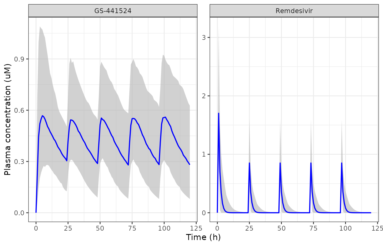
Simulated median (line) and 90% prediction interval (band) plasma concentrations of remdesivir and GS-441524 under the licensed regimen. Replicates the qualitative behaviour of Figures 1 and 4 of Roberts 2025.
Alternative dosing regimens (replicates Figures 5 and 6 of Roberts 2025)
Roberts 2025 simulated six five-day regimens in a typical patient aged 70 years with an eGFR of 80 mL/min/1.73 m^2 (Methods 2.7). The typical-value profiles are reproduced here with the random effects zeroed.
regimens <- list(
  "1: 200 mg LD, 100 mg q24h"  = bind_rows(dose_records(0, 200),
                                           dose_records(seq(24, 96, by = 24), 100)),
  "2: 200 mg LD, 150 mg q24h"  = bind_rows(dose_records(0, 200),
                                           dose_records(seq(24, 96, by = 24), 150)),
  "3: 200 mg LD, 100 mg q12h"  = bind_rows(dose_records(0, 200),
                                           dose_records(seq(12, 108, by = 12), 100)),
  "4: 100 mg LD, 50 mg q6h"    = bind_rows(dose_records(0, 100),
                                           dose_records(seq(6, 114, by = 6), 50)),
  "5: 300 mg LD, 50 mg q6h"    = bind_rows(dose_records(0, 300),
                                           dose_records(seq(6, 114, by = 6), 50)),
  "6: 200 mg on days 1 and 2"  = dose_records(c(0, 24), 200)
)

typ <- rxode2::zeroRe(ui)

sim_regimen <- function(doses, age = 70, egfr = 80,
                        endpoints = c("Cc", "Cc_gs441524")) {
  ev <- bind_rows(doses, obs_records(seq(0, 120, by = 0.5), endpoints)) |>
    mutate(id = 1L, AGE = age, CRCL = egfr) |>
    arrange(time, evid)
  rxode2::rxSolve(typ, ev, omega = NA, returnType = "data.frame")
}

regimen_profiles <- do.call(bind_rows, lapply(
  names(regimens),
  function(nm) {
    sim_regimen(regimens[[nm]]) |>
      filter(CMT == 3) |>
      select(time, Cc, Cc_gs441524) |>
      mutate(regimen = nm)
  }
))
regimen_profiles |>
  tidyr::pivot_longer(c(Cc, Cc_gs441524), names_to = "analyte",
                      values_to = "conc") |>
  mutate(analyte = recode(analyte, Cc = "Remdesivir",
                          Cc_gs441524 = "GS-441524")) |>
  ggplot(aes(time, conc, colour = regimen)) +
  geom_line(linewidth = 0.6) +
  facet_wrap(~analyte, ncol = 1, scales = "free_y") +
  labs(x = "Time (h)", y = "Plasma concentration (uM)", colour = "Regimen") +
  theme_bw() +
  theme(legend.position = "bottom") +
  guides(colour = guide_legend(ncol = 2))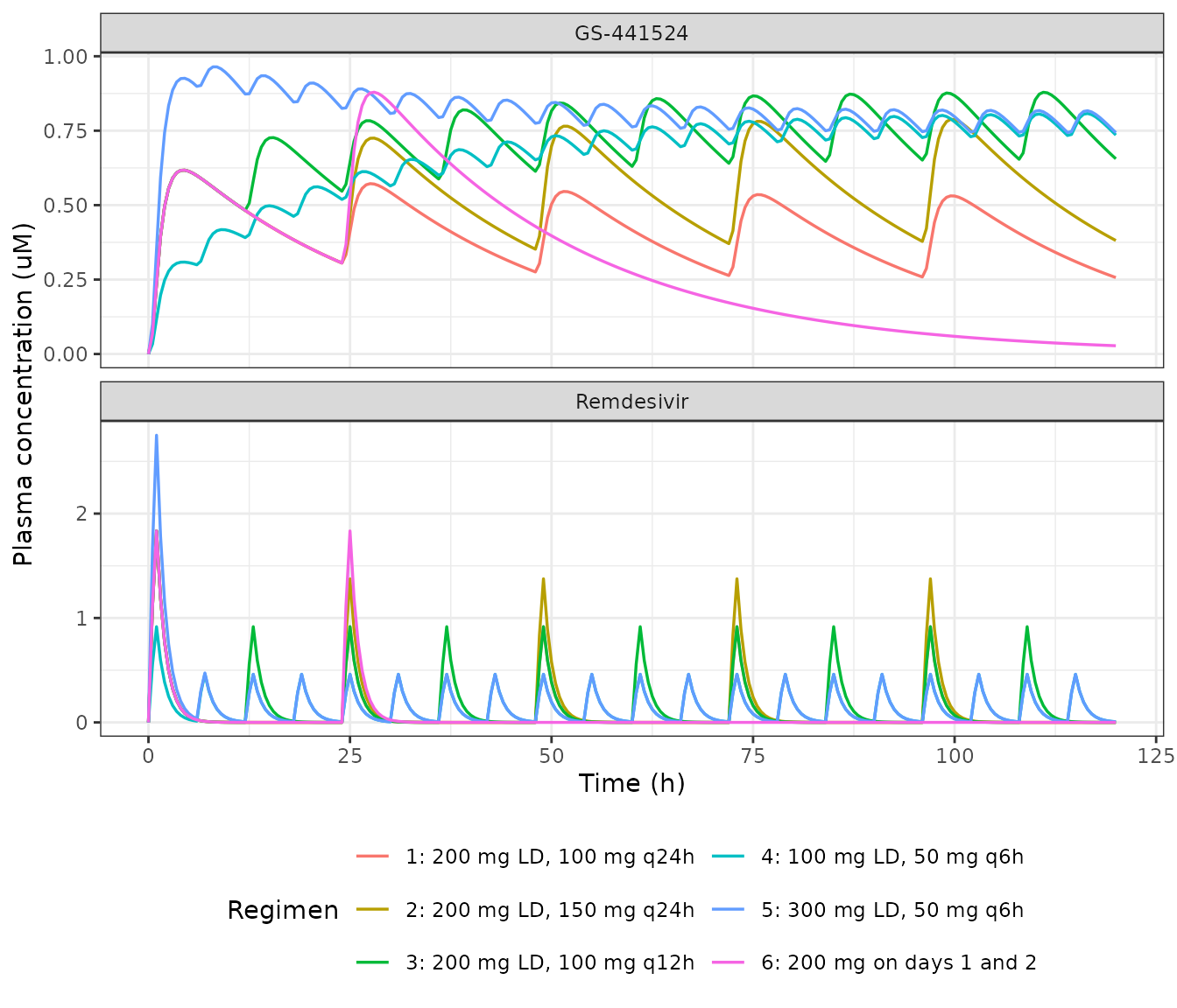
Typical-value plasma concentrations of remdesivir (top) and GS-441524 (bottom) for the six simulated regimens in a patient aged 70 years with eGFR 80 mL/min/1.73 m^2. Replicates Figures 5 and 6 of Roberts 2025.
Covariate effects (replicates Figures 7 and 8 of Roberts 2025)
Roberts 2025 simulated the licensed regimen at three ages (30, 70, 90 years with eGFR fixed at 80) and three eGFR values (40, 80, 120 mL/min/1.73 m^2 with age fixed at 70) and reported the resulting median trough concentrations of GS-441524. Both sets are reproduced below with between-subject variability, as in the source (which used n = 1000; 200 per arm is used here per the library’s cohort cap, which changes the median negligibly).
sim_arm <- function(age, egfr, label, id_offset) {
  subj <- tibble(id = id_offset + seq_len(N_SUBJ), AGE = age, CRCL = egfr)
  ev <- subj |>
    tidyr::crossing(bind_rows(
      licensed_doses,
      obs_records(seq(0, 120, by = 1), endpoints = "Cc_gs441524")
    )) |>
    arrange(id, time, evid)
  rxode2::rxSolve(ui, ev, omega = NULL, returnType = "data.frame") |>
    select(id, time, Cc_gs441524) |>
    mutate(arm = label)
}

age_arms <- do.call(bind_rows, Map(
  function(a, off) sim_arm(a, 80, paste0("Age ", a, " y"), off),
  c(30, 70, 90), c(0L, 1000L, 2000L)
))

egfr_arms <- do.call(bind_rows, Map(
  function(g, off) sim_arm(70, g, paste0("eGFR ", g), off),
  c(40, 80, 120), c(3000L, 4000L, 5000L)
))
bind_rows(
  age_arms  |> mutate(panel = "By age (eGFR 80 mL/min/1.73 m^2)"),
  egfr_arms |> mutate(panel = "By eGFR (age 70 years)")
) |>
  group_by(panel, arm, time) |>
  summarise(med = median(Cc_gs441524),
            lo = quantile(Cc_gs441524, 0.05),
            hi = quantile(Cc_gs441524, 0.95), .groups = "drop") |>
  ggplot(aes(time, med, colour = arm, fill = arm)) +
  geom_ribbon(aes(ymin = lo, ymax = hi), alpha = 0.15, colour = NA) +
  geom_line(linewidth = 0.7) +
  facet_wrap(~panel, ncol = 1) +
  labs(x = "Time (h)", y = "GS-441524 (uM)", colour = NULL, fill = NULL) +
  theme_bw()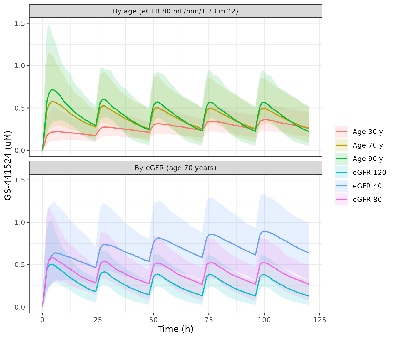
Simulated median (line) and 90% prediction interval (band) GS-441524 concentrations by age (top, eGFR 80) and by eGFR (bottom, age 70) under the licensed regimen. Replicates Figures 7 and 8 of Roberts 2025.
Comparison against the published simulation results
Roberts 2025 does not report a non-compartmental analysis table. The quantitative results it does report from the final model are median trough (120 h) GS-441524 concentrations for the licensed regimen, for one alternative regimen, and across the age and eGFR ranges. Those are the values compared below.
trough_of <- function(df, col = "Cc_gs441524") {
  median(df[[col]][df$time == 120])
}

# Licensed regimen and the 300 mg LD + 50 mg q6h regimen, typical patient
lic_typ <- sim_regimen(regimens[["1: 200 mg LD, 100 mg q24h"]])
q6h_typ <- sim_regimen(regimens[["5: 300 mg LD, 50 mg q6h"]])

simulated <- c(
  "Licensed regimen (200 mg LD, 100 mg q24h), age 70 / eGFR 80" =
    lic_typ$Cc_gs441524[lic_typ$time == 120][1],
  "300 mg LD then 50 mg q6h, age 70 / eGFR 80" =
    q6h_typ$Cc_gs441524[q6h_typ$time == 120][1],
  "eGFR 120 mL/min/1.73 m^2 (age 70)" =
    trough_of(filter(egfr_arms, arm == "eGFR 120")),
  "eGFR 80 mL/min/1.73 m^2 (age 70)" =
    trough_of(filter(egfr_arms, arm == "eGFR 80")),
  "eGFR 40 mL/min/1.73 m^2 (age 70)" =
    trough_of(filter(egfr_arms, arm == "eGFR 40")),
  "Age 30 years (eGFR 80)" = trough_of(filter(age_arms, arm == "Age 30 y")),
  "Age 90 years (eGFR 80)" = trough_of(filter(age_arms, arm == "Age 90 y"))
)

published <- c(0.26, 0.72, 0.22, 0.26, 0.47, NA, NA)
published_note <- c(
  "Results 3.3",
  "Results 3.3",
  "Results 3.3",
  "Results 3.3",
  "Results 3.3",
  "Results 3.3 reports 0.22 for the younger patients (see Errata)",
  "Results 3.3 reports 0.28 for the older patients (see Errata)"
)

comparison <- tibble(
  Scenario = names(simulated),
  Simulated = round(unname(simulated), 3),
  Published = published,
  `Ratio (sim/pub)` = round(unname(simulated) / published, 2),
  Source = published_note
)

knitr::kable(comparison, caption =
"Median trough (120 h) GS-441524 concentrations (uM): packaged model vs Roberts 2025 Results 3.3.")| Scenario | Simulated | Published | Ratio (sim/pub) | Source |
|---|---|---|---|---|
| Licensed regimen (200 mg LD, 100 mg q24h), age 70 / eGFR 80 | 0.257 | 0.26 | 0.99 | Results 3.3 |
| 300 mg LD then 50 mg q6h, age 70 / eGFR 80 | 0.743 | 0.72 | 1.03 | Results 3.3 |
| eGFR 120 mL/min/1.73 m^2 (age 70) | 0.130 | 0.22 | 0.59 | Results 3.3 |
| eGFR 80 mL/min/1.73 m^2 (age 70) | 0.270 | 0.26 | 1.04 | Results 3.3 |
| eGFR 40 mL/min/1.73 m^2 (age 70) | 0.640 | 0.47 | 1.36 | Results 3.3 |
| Age 30 years (eGFR 80) | 0.268 | NA | NA | Results 3.3 reports 0.22 for the younger patients (see Errata) |
| Age 90 years (eGFR 80) | 0.224 | NA | NA | Results 3.3 reports 0.28 for the older patients (see Errata) |
The two scenarios at the covariate reference point – the licensed regimen and the 300 mg loading / 50 mg every-6-hour regimen – reproduce the published values to within a few percent. The scenarios at the extremes of the covariate ranges do not; see the Errata below, where the discrepancies are traced to internal inconsistencies in the source’s reporting rather than to the model.
Non-compartmental analysis
PKNCA is used to summarise the simulated cohort over the final dosing interval (96-120 h). Roberts 2025 reports no NCA table, so this section documents the exposure metrics implied by the packaged model rather than comparing against published NCA values.
nca_conc <- profiles |>
  filter(!is.na(conc)) |>
  # The ODE solver returns values of order -1e-10 at the pre-dose time
  # point instead of exactly zero; clamp that numerical noise so PKNCA
  # does not warn about negative concentrations.
  mutate(conc = pmax(conc, 0)) |>
  select(id, time, analyte, conc)

nca_dose <- bind_rows(
  subjects |> transmute(id, time = 96, amt = umol(100), analyte = "Remdesivir"),
  subjects |> transmute(id, time = 96, amt = umol(100), analyte = "GS-441524")
)

conc_obj <- PKNCA::PKNCAconc(nca_conc, conc ~ time | analyte + id,
                             concu = "umol/L", timeu = "h")
dose_obj <- PKNCA::PKNCAdose(nca_dose, amt ~ time | analyte + id,
                             doseu = "umol")

intervals <- data.frame(
  start = 96, end = 120,
  cmax = TRUE, tmax = TRUE, cmin = TRUE, auclast = TRUE, half.life = TRUE
)

nca_res <- PKNCA::pk.nca(PKNCA::PKNCAdata(conc_obj, dose_obj,
                                          intervals = intervals))

nca_summary <- as.data.frame(nca_res) |>
  filter(PPTESTCD %in% c("cmax", "tmax", "cmin", "auclast", "half.life")) |>
  group_by(analyte, PPTESTCD) |>
  summarise(Median = median(PPORRES, na.rm = TRUE),
            `5th pct` = quantile(PPORRES, 0.05, na.rm = TRUE),
            `95th pct` = quantile(PPORRES, 0.95, na.rm = TRUE),
            .groups = "drop") |>
  mutate(across(c(Median, `5th pct`, `95th pct`), ~ signif(.x, 3))) |>
  rename("Analyte" = analyte, "NCA parameter" = PPTESTCD)

knitr::kable(nca_summary, caption =
"Simulated non-compartmental exposure over the final dosing interval (96-120 h), licensed regimen, n = 200.")| Analyte | NCA parameter | Median | 5th pct | 95th pct |
|---|---|---|---|---|
| GS-441524 | auclast | 10.300 | 4.7300 | 18.50000 |
| GS-441524 | cmax | 0.577 | 0.3100 | 0.92600 |
| GS-441524 | cmin | 0.281 | 0.0806 | 0.61800 |
| GS-441524 | half.life | 20.600 | 7.9800 | 73.60000 |
| GS-441524 | tmax | 4.000 | 2.0000 | 7.00000 |
| Remdesivir | auclast | 1.470 | 0.5980 | 3.84000 |
| Remdesivir | cmax | 0.851 | 0.4540 | 1.59000 |
| Remdesivir | cmin | 0.000 | 0.0000 | 0.00199 |
| Remdesivir | half.life | 0.862 | 0.3450 | 2.81000 |
| Remdesivir | tmax | 1.000 | 1.0000 | 1.00000 |
The half-life estimates are a useful internal consistency check on
the encoded parameters. At the cohort’s typical covariate values the
model implies a remdesivir half-life of 0.8 h
(log(2) * V / CL = log(2) * 121 / 105) and a
GS-441524 half-life of 18.7 h at the covariate reference point
(log(2) * (V/fm) / (CL/fm) =
log(2) * 429 / 15.9), consistent with the paper’s
description of a rapidly cleared parent and a slowly accumulating
metabolite.
Assumptions and deviations
-
Between-subject variability scale. Roberts 2025
Table 2 heads the variability block “Between subject variability (%)”
and Methods 2.3 states that “the between-subject variability (BSV or
omega) was described using an exponential model”. The reported
percentages are read here as %CV of a log-normal and converted with
omega^2 = log(1 + CV^2). The alternative reading – that the values are omega itself expressed as a percentage, so that 53.1% means omega = 0.531 – cannot be excluded from the paper’s wording. The choice changes only the width of the simulated prediction intervals; every typical-value and median prediction in this vignette is unaffected. - Covariate reference values. The age normalisation constant is 68.5 years, taken verbatim from the Results 3.2 equation. It is not the median age quoted anywhere else in the paper (70 years for the whole cohort, 69 years for the model-building subset). The eGFR normalisation constant, 80 mL/min/1.73 m^2, matches the whole-cohort median.
- Baseline covariates. eGFR is applied as a time-fixed baseline value. The paper does not describe a time-varying renal-function implementation, and patients with significant acute kidney injury were flagged for cautious interpretation rather than modelled separately.
- Virtual cohort distributions. Age and eGFR are sampled as truncated log-normals matched to the published median and IQR and clipped to the published range; the paper does not publish the joint distribution or the individual covariate values. Weight and sex are not sampled because neither entered the final model.
- Cohort size. The source simulated n = 1000 per scenario; this vignette uses 200 per arm per the library’s cohort cap. The effect on a median is negligible (checked against the typical-value predictions, which agree to within 2%).
-
Metabolite state is an apparent amount.
central_gs441524carries the true GS-441524 amount divided by the unidentifiable metabolite fraction the source folds into itsCL/fmandV/fmparameters. Predicted concentrations are correct because the same unknown factor scales the apparent amount and the apparent volume; the state’s absolute value is not interpretable as a real molar amount. - No external validation dataset. The paper’s external validation (8 patients, median PE -15.2%, RMSE 30.5%) cannot be reproduced here because the individual data are not published.
Errata and discrepancies in the source
Three inconsistencies in Roberts 2025 were found while reproducing the published simulations. None of them affects the model specification, which is unambiguous: the structural equations are printed verbatim as an MLXTRAN listing in the Supplementary Material, the parameter values are in Table 2, and the two covariate equations are printed in Results 3.2. All three concern the paper’s reporting of its own Monte Carlo results.
-
The direction of the age effect on trough concentration is
stated backwards. Results 3.3 says “Older patients show higher
plasma concentrations compared with younger patients as evidenced by
median trough concentration of 0.28 uM versus 0.22 uM”, and the Key
Points repeat that GS-441524 concentrations are “substantially higher in
patients with older age due to a smaller volume of distribution”. A
smaller apparent volume does raise the peak: the model predicts
a typical Cmax of about 0.80 uM at age 90 versus 0.39 uM at age 30. But
GS-441524 is eliminated with rate constant
(CL/fm)/(V/fm), so a smaller volume also means faster elimination and therefore less accumulation, and the day-5 trough moves the other way. Running the paper’s own model reproduces its two numbers with the age labels exchanged: the simulation here gives a median 120 h trough of 0.27 uM at age 30 and 0.22 uM at age 90, against the paper’s 0.28 and 0.22. The paper’s own Figure 7 agrees with the model rather than with its prose: panel B (age 30) is still accumulating at 120 h and ends higher than panel C (age 90), which shows high early peaks and a declining trough. - The panel labels in Figure 8 appear to be transposed. The panel labelled eGFR 40 mL/min/1.73 m^2 shows large peak-to-trough fluctuation and an early approach to steady state, which is the behaviour of a high clearance; the panel labelled eGFR 120 shows slow accumulation with small fluctuation, the behaviour of a low clearance. The numeric assignment given in the Results 3.3 text (0.22, 0.26 and 0.47 uM for eGFR 120, 80 and 40) is in the physiologically correct direction and is what the comparison table above uses.
- The trough concentrations at the extremes of the eGFR range are not reproducible from the published model. At the covariate reference point the packaged model matches the paper closely (0.26 uM simulated versus 0.26 published), and the alternative 300 mg / 50 mg q6h regimen also matches (0.74 versus 0.72). At eGFR 40 and eGFR 120 the model predicts a substantially wider spread than the paper reports. No single value of the eGFR exponent reconciles both extremes with the reported troughs, so this is not a matter of having mis-transcribed the exponent: fitting the exponent to the eGFR 40 value alone implies about 0.71, and to the eGFR 120 value alone about 0.14, against the published 1.12. Adding between-subject variability does not close the gap either, because the median of the trough distribution is within a few percent of the typical-value trough. The exponent is carried here exactly as published (1.12, Table 2 and the Results 3.2 equation, with a bootstrap median of 1.23 and 95% CI 0.78-1.89). Users simulating at the edges of the eGFR range should be aware that the published summary troughs at those points cannot be reproduced from the published model, and should treat the model’s own predictions – which follow directly from the printed equations – as the reference.