Inhaled fluticasone propionate (Weber 2015)
Source:vignettes/articles/Weber_2015_fluticasone_inhaled.Rmd
Weber_2015_fluticasone_inhaled.RmdModel and source
- Citation: Weber B, Hochhaus G. (2015). A Systematic Analysis of the Sensitivity of Plasma Pharmacokinetics to Detect Differences in the Pulmonary Performance of Inhaled Fluticasone Propionate Products Using a Model-Based Simulation Approach. AAPS J 17(4):999-1010.
- Article: https://doi.org/10.1208/s12248-015-9768-y
mod_meta <- rxode2::rxode(readModelDb("Weber_2015_fluticasone_inhaled"))
#> ℹ parameter labels from comments will be replaced by 'label()'
mod_meta$description
#> [1] "Semi-mechanistic. Population PK model for inhaled fluticasone propionate (FP) in healthy adult volunteers (Weber 2015), used for Monte-Carlo simulation of PK-based bioequivalence trials. Separate central (LC1 -> LC2) and peripheral (LP1 -> LP2) lung deposition compartments hold undissolved drug particles (LC1, LP1) and dissolved drug (LC2, LP2); mucociliary clearance kmuc removes undissolved particles from central lung regions only; dissolved drug is absorbed into a two-compartment systemic disposition with central-to-peripheral rate constants k12 and k21. Each administration splits across LC1 (bioavailability flung * fc) and LP1 (bioavailability flung * (1 - fc)); the remaining (1 - flung) fraction is assumed to have negligible oral bioavailability. F_Lung and F_C are logit-transformed; all other parameters are log-transformed. Structural parameters and BSV were taken from the validated FP inhalation model of Weber and Hochhaus 2013 (reference 13 of Weber 2015); BOV on F_Lung, F_C, and kmuc described as a paper-specific extension for crossover-trial simulation is NOT encoded in this model file (see vignette Assumptions and deviations)."
mod_meta$reference
#> [1] "Weber B, Hochhaus G. (2015). A Systematic Analysis of the Sensitivity of Plasma Pharmacokinetics to Detect Differences in the Pulmonary Performance of Inhaled Fluticasone Propionate Products Using a Model-Based Simulation Approach. AAPS J 17(4):999-1010. doi:10.1208/s12248-015-9768-y."
mod_meta$units
#> $time
#> [1] "hour"
#>
#> $dosing
#> [1] "ug"
#>
#> $concentration
#> [1] "ng/mL"
Population
Weber 2015 is a Monte-Carlo simulation study; the underlying structural model, typical parameter values, and between-subject variability (BSV) terms were taken from the previously validated FP inhalation model of Weber and Hochhaus 2013 (Mol Pharm 10(8):2873-85; reference 13 of Weber 2015). That upstream model was fit to clinically observed FP plasma concentrations in healthy adult volunteers across four inhaled corticosteroids; the typical adult demographics of those source studies are not reproduced in detail in Weber 2015 because the present paper does not fit observed plasma concentrations. The simulation experiment of Weber 2015 uses three series of trials with single-dose two-period crossover designs: Series 1 evaluates 10, 20, 30, 40, 50, 60, and 70 subjects with identical test (T) and reference (R) inhalers (testing different lots of the R product against each other); Series 2 evaluates 50, 100, and 200 subjects per T-vs-R comparison across 60 different T products that each differ from R in only one of three pulmonary performance parameters (F_Lung, F_C, k_diss); Series 3 evaluates 50, 100, and 200 subjects per T-vs-R comparison across 343 T products that differ in all three parameters simultaneously.
The same metadata is available programmatically via
readModelDb("Weber_2015_fluticasone_inhaled")$population.
Source trace
The per-parameter origin is recorded as an in-file comment next to
each ini() entry in
inst/modeldb/specificDrugs/Weber_2015_fluticasone_inhaled.R.
The table below collects them in one place for review.
| Equation / parameter | Value | Source location |
|---|---|---|
logitflung (logit F_Lung) |
log(0.16 / 0.84) | Weber 2015 Table I: F_Lung = 0.16 (FP Diskus reference) |
logitfc (logit F_C) |
log(0.5 / 0.5) = 0 | Weber 2015 Table I: F_C = 0.50 |
lkdiss (log k_diss) |
log(0.189) | Weber 2015 Table I: k_diss = 0.189 1/h |
lkmuc (log k_muc) |
log(0.938) | Weber 2015 Table I: k_muc = 0.938 1/h |
lkpulc (log k_pul,C) |
log(10) | Weber 2015 Table I: k_pul,C = 10 1/h |
lkpulp (log k_pul,P) |
log(20) | Weber 2015 Table I: k_pul,P = 20 1/h |
lcl (log CL) |
log(73) | Weber 2015 Table I: CL = 73 L/h |
lvc (log V_C) |
log(31) | Weber 2015 Table I: V_C = 31 L |
lk12 (log k12) |
log(1.78) | Weber 2015 Table I: k12 = 1.78 1/h |
lk21 (log k21) |
log(0.09) | Weber 2015 Table I: k21 = 0.09 1/h |
| All BSV variances (10 parameters) | omega^2 = log(1 + 0.30^2) ~= 0.0862 | Weber 2015 Table I: “Between-subject variability (CV) (%)” column = 30% for every parameter |
propSd (proportional residual SD) |
0.20 | Weber 2015 Table I footer: “Residual variability was 20%” |
| Lung deposition compartments LC1 / LC2 / LP1 / LP2 | n/a | Weber 2015 Fig. 1 and caption |
| Mucociliary clearance on LC1 only (no kmuc on LP1) | n/a | Weber 2015 Methods, “Pharmacokinetic Model” first paragraph |
| Dose split: f(LC1) = flung * fc, f(LP1) = flung * (1 - fc) | n/a | Weber 2015 Fig. 1 caption |
| Logit transformation for F_Lung and F_C | n/a | Weber 2015 Methods, paragraph after Fig. 1 |
| Sampling schedule used in Weber 2015 trial simulations | 0.25, 0.5, 0.75, 1, 1.5, 2, 3, 4, 5, 6, 8, 10, 12, 24, 36, 48 h | Weber 2015 Methods, “Series 1” final sentence |
Virtual cohort
Weber 2015 simulates inhaled FP plasma profiles for healthy adult volunteers. The paper does not specify an absolute dose magnitude (the PK model is scale-invariant in the emitted dose, so reproducing the paper’s reported T/R ratios is independent of dose). For demonstration the cohort below uses a single 500 ug inhaled dose, which is in the clinical range of FP Diskus per-actuation doses (100, 250, or 500 ug); the cohort size of 50 matches Series 1 of Weber 2015 and is the sample size shown to achieve approximately 90% statistical power for bioequivalence with a 90% confidence-interval acceptance range of 80%-125% (Weber 2015 Results, “Series 1” paragraph). The observation grid reproduces the sampling schedule from Weber 2015 Methods (“Series 1” final sentence).
set.seed(20260603)

n_subjects <- 50L
dose_ug    <- 500
obs_times  <- c(0.25, 0.5, 0.75, 1, 1.5, 2, 3, 4, 5, 6, 8, 10, 12, 24, 36, 48)

# Each administration enters as TWO simultaneous dose rows (cmt = LC1
# and cmt = LP1, both with amt = total emitted dose). The
# bioavailabilities f(LC1) = flung * fc and f(LP1) = flung * (1 - fc)
# defined in the model file split the emitted dose into the central-
# and peripheral-lung regions.
make_events_one_product <- function(n, id_offset = 0L, product_label) {
  ids <- id_offset + seq_len(n)
  dose_lc1 <- tibble(id = ids, time = 0, amt = dose_ug, cmt = "LC1", evid = 1L)
  dose_lp1 <- tibble(id = ids, time = 0, amt = dose_ug, cmt = "LP1", evid = 1L)
  obs      <- tidyr::expand_grid(id = ids, time = obs_times) |>
    dplyr::mutate(amt = 0, cmt = "central", evid = 0L)
  dplyr::bind_rows(dose_lc1, dose_lp1, obs) |>
    dplyr::mutate(product = product_label) |>
    dplyr::arrange(id, time, dplyr::desc(evid))
}

events_ref <- make_events_one_product(n_subjects, id_offset = 0L, "Reference")
stopifnot(!anyDuplicated(unique(events_ref[, c("id", "time", "evid")])))

cat("Subjects:", n_subjects,
    " | Dose rows:", sum(events_ref$evid == 1L),
    " | Observation rows:", sum(events_ref$evid == 0L), "\n")
#> Subjects: 50  | Dose rows: 100  | Observation rows: 800
Simulation
mod <- readModelDb("Weber_2015_fluticasone_inhaled")

sim_ref <- rxode2::rxSolve(
  mod,
  events = events_ref,
  keep   = c("product")
) |>
  as.data.frame()
#> ℹ parameter labels from comments will be replaced by 'label()'

cat("Cc range across cohort:", round(range(sim_ref$Cc, na.rm = TRUE), 4),
    "ng/mL\n")
#> Cc range across cohort: 1e-04 0.2528 ng/mL
For deterministic typical-value replication (Figure 2 of Weber 2015 shows the typical plasma profile when both T and R are the FP Diskus inhaler), zero out the random effects:
mod_typical <- mod |> rxode2::zeroRe()
#> ℹ parameter labels from comments will be replaced by 'label()'

events_typical <- tibble(
  id = 1L, time = 0, amt = dose_ug, cmt = "LC1", evid = 1L
) |>
  dplyr::bind_rows(
    tibble(id = 1L, time = 0, amt = dose_ug, cmt = "LP1", evid = 1L)
  ) |>
  dplyr::bind_rows(
    tibble(id = 1L, time = obs_times, amt = 0, cmt = "central", evid = 0L)
  ) |>
  dplyr::arrange(id, time, dplyr::desc(evid))

sim_typical <- rxode2::rxSolve(mod_typical, events = events_typical) |>
  as.data.frame()
#> ℹ omega/sigma items treated as zero: 'etalogitflung', 'etalogitfc', 'etalkdiss', 'etalkmuc', 'etalkpulc', 'etalkpulp', 'etalcl', 'etalvc', 'etalk12', 'etalk21'
Replicate published figures
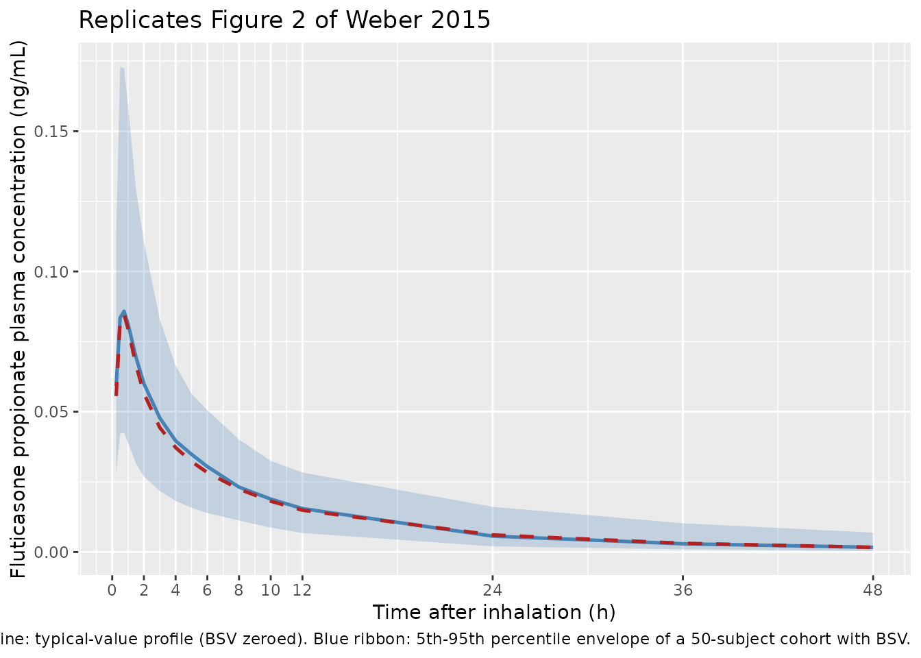
Figure 2 – typical plasma profile for the FP Diskus reference product
Weber 2015 Figure 2 displays representative simulated plasma concentration-time profiles for the test (T) and reference (R) products when both are the FP Diskus inhaler (testing different batches of R against each other). The chunk below renders the typical-value (no BSV) profile for the FP Diskus reference product and overlays the simulated 5th / 50th / 95th-percentile envelope from the 50-subject cohort with BSV.
cohort_summary <- sim_ref |>
  dplyr::filter(time > 0) |>
  dplyr::group_by(time) |>
  dplyr::summarise(
    Q05 = quantile(Cc, 0.05, na.rm = TRUE),
    Q50 = quantile(Cc, 0.50, na.rm = TRUE),
    Q95 = quantile(Cc, 0.95, na.rm = TRUE),
    .groups = "drop"
  )

typical_curve <- sim_typical |>
  dplyr::filter(time > 0) |>
  dplyr::select(time, Cc)

ggplot() +
  geom_ribbon(
    data = cohort_summary,
    aes(time, ymin = Q05, ymax = Q95),
    alpha = 0.25, fill = "steelblue"
  ) +
  geom_line(data = cohort_summary, aes(time, Q50), colour = "steelblue", linewidth = 0.9) +
  geom_line(data = typical_curve,  aes(time, Cc),  colour = "firebrick", linewidth = 0.9, linetype = "dashed") +
  scale_x_continuous(breaks = c(0, 2, 4, 6, 8, 10, 12, 24, 36, 48)) +
  labs(
    x = "Time after inhalation (h)",
    y = "Fluticasone propionate plasma concentration (ng/mL)",
    title = "Replicates Figure 2 of Weber 2015",
    caption = paste("Single 500 ug inhaled dose of the FP Diskus reference product.",
                    "Dashed red line: typical-value profile (BSV zeroed).",
                    "Blue ribbon: 5th-95th percentile envelope of a 50-subject cohort with BSV.")
  )
PKNCA validation
Compute Cmax, Tmax, AUC over 0-48 h, and AUC over 0-Inf per subject with PKNCA, using the virtual cohort defined above. Weber 2015 Methods footnote 1 notes that AUC0-48 covered at least 80% of AUC0-Inf for these simulations.
sim_nca <- sim_ref |>
  dplyr::filter(!is.na(Cc), time > 0) |>
  dplyr::select(id, time, Cc, product)

dose_df <- events_ref |>
  dplyr::filter(evid == 1L, cmt == "LC1") |>          # one row per administration per subject
  dplyr::mutate(amt = dose_ug) |>
  dplyr::select(id, time, amt, product)

conc_obj <- PKNCA::PKNCAconc(
  sim_nca, Cc ~ time | product + id,
  concu = "ng/mL", timeu = "h"
)
dose_obj <- PKNCA::PKNCAdose(
  dose_df, amt ~ time | product + id,
  doseu = "ug"
)

intervals <- data.frame(
  start      = 0,
  end        = c(48, Inf),
  cmax       = c(TRUE, FALSE),
  tmax       = c(TRUE, FALSE),
  auclast    = c(TRUE, FALSE),
  aucinf.obs = c(FALSE, TRUE)
)

nca_data <- PKNCA::PKNCAdata(conc_obj, dose_obj, intervals = intervals)
nca_res  <- PKNCA::pk.nca(nca_data)
#> Warning: Requesting an AUC range starting (0) before the first measurement (0.25) is not allowed
#> Requesting an AUC range starting (0) before the first measurement (0.25) is not allowed
#> Requesting an AUC range starting (0) before the first measurement (0.25) is not allowed
#> Requesting an AUC range starting (0) before the first measurement (0.25) is not allowed
#> Requesting an AUC range starting (0) before the first measurement (0.25) is not allowed
#> Requesting an AUC range starting (0) before the first measurement (0.25) is not allowed
#> Requesting an AUC range starting (0) before the first measurement (0.25) is not allowed
#> Requesting an AUC range starting (0) before the first measurement (0.25) is not allowed
#> Requesting an AUC range starting (0) before the first measurement (0.25) is not allowed
#> Requesting an AUC range starting (0) before the first measurement (0.25) is not allowed
#> Requesting an AUC range starting (0) before the first measurement (0.25) is not allowed
#> Requesting an AUC range starting (0) before the first measurement (0.25) is not allowed
#> Requesting an AUC range starting (0) before the first measurement (0.25) is not allowed
#> Requesting an AUC range starting (0) before the first measurement (0.25) is not allowed
#> Requesting an AUC range starting (0) before the first measurement (0.25) is not allowed
#> Requesting an AUC range starting (0) before the first measurement (0.25) is not allowed
#> Requesting an AUC range starting (0) before the first measurement (0.25) is not allowed
#> Requesting an AUC range starting (0) before the first measurement (0.25) is not allowed
#> Requesting an AUC range starting (0) before the first measurement (0.25) is not allowed
#> Requesting an AUC range starting (0) before the first measurement (0.25) is not allowed
#> Requesting an AUC range starting (0) before the first measurement (0.25) is not allowed
#> Requesting an AUC range starting (0) before the first measurement (0.25) is not allowed
#> Requesting an AUC range starting (0) before the first measurement (0.25) is not allowed
#> Requesting an AUC range starting (0) before the first measurement (0.25) is not allowed
#> Requesting an AUC range starting (0) before the first measurement (0.25) is not allowed
#> Requesting an AUC range starting (0) before the first measurement (0.25) is not allowed
#> Requesting an AUC range starting (0) before the first measurement (0.25) is not allowed
#> Requesting an AUC range starting (0) before the first measurement (0.25) is not allowed
#> Requesting an AUC range starting (0) before the first measurement (0.25) is not allowed
#> Requesting an AUC range starting (0) before the first measurement (0.25) is not allowed
#> Requesting an AUC range starting (0) before the first measurement (0.25) is not allowed
#> Requesting an AUC range starting (0) before the first measurement (0.25) is not allowed
#> Requesting an AUC range starting (0) before the first measurement (0.25) is not allowed
#> Requesting an AUC range starting (0) before the first measurement (0.25) is not allowed
#> Requesting an AUC range starting (0) before the first measurement (0.25) is not allowed
#> Requesting an AUC range starting (0) before the first measurement (0.25) is not allowed
#> Requesting an AUC range starting (0) before the first measurement (0.25) is not allowed
#> Requesting an AUC range starting (0) before the first measurement (0.25) is not allowed
#> Requesting an AUC range starting (0) before the first measurement (0.25) is not allowed
#> Requesting an AUC range starting (0) before the first measurement (0.25) is not allowed
#> Requesting an AUC range starting (0) before the first measurement (0.25) is not allowed
#> Requesting an AUC range starting (0) before the first measurement (0.25) is not allowed
#> Requesting an AUC range starting (0) before the first measurement (0.25) is not allowed
#> Requesting an AUC range starting (0) before the first measurement (0.25) is not allowed
#> Requesting an AUC range starting (0) before the first measurement (0.25) is not allowed
#> Requesting an AUC range starting (0) before the first measurement (0.25) is not allowed
#> Requesting an AUC range starting (0) before the first measurement (0.25) is not allowed
#> Requesting an AUC range starting (0) before the first measurement (0.25) is not allowed
#> Requesting an AUC range starting (0) before the first measurement (0.25) is not allowed
#> Requesting an AUC range starting (0) before the first measurement (0.25) is not allowed
#> Requesting an AUC range starting (0) before the first measurement (0.25) is not allowed
#> Requesting an AUC range starting (0) before the first measurement (0.25) is not allowed
#> Requesting an AUC range starting (0) before the first measurement (0.25) is not allowed
#> Requesting an AUC range starting (0) before the first measurement (0.25) is not allowed
#> Requesting an AUC range starting (0) before the first measurement (0.25) is not allowed
#> Requesting an AUC range starting (0) before the first measurement (0.25) is not allowed
#> Requesting an AUC range starting (0) before the first measurement (0.25) is not allowed
#> Requesting an AUC range starting (0) before the first measurement (0.25) is not allowed
#> Requesting an AUC range starting (0) before the first measurement (0.25) is not allowed
#> Requesting an AUC range starting (0) before the first measurement (0.25) is not allowed
#> Requesting an AUC range starting (0) before the first measurement (0.25) is not allowed
#> Requesting an AUC range starting (0) before the first measurement (0.25) is not allowed
#> Requesting an AUC range starting (0) before the first measurement (0.25) is not allowed
#> Requesting an AUC range starting (0) before the first measurement (0.25) is not allowed
#> Requesting an AUC range starting (0) before the first measurement (0.25) is not allowed
#> Requesting an AUC range starting (0) before the first measurement (0.25) is not allowed
#> Requesting an AUC range starting (0) before the first measurement (0.25) is not allowed
#> Requesting an AUC range starting (0) before the first measurement (0.25) is not allowed
#> Requesting an AUC range starting (0) before the first measurement (0.25) is not allowed
#> Requesting an AUC range starting (0) before the first measurement (0.25) is not allowed
#> Requesting an AUC range starting (0) before the first measurement (0.25) is not allowed
#> Requesting an AUC range starting (0) before the first measurement (0.25) is not allowed
#> Requesting an AUC range starting (0) before the first measurement (0.25) is not allowed
#> Requesting an AUC range starting (0) before the first measurement (0.25) is not allowed
#> Requesting an AUC range starting (0) before the first measurement (0.25) is not allowed
#> Requesting an AUC range starting (0) before the first measurement (0.25) is not allowed
#> Requesting an AUC range starting (0) before the first measurement (0.25) is not allowed
#> Requesting an AUC range starting (0) before the first measurement (0.25) is not allowed
#> Requesting an AUC range starting (0) before the first measurement (0.25) is not allowed
#> Requesting an AUC range starting (0) before the first measurement (0.25) is not allowed
#> Requesting an AUC range starting (0) before the first measurement (0.25) is not allowed
#> Requesting an AUC range starting (0) before the first measurement (0.25) is not allowed
#> Requesting an AUC range starting (0) before the first measurement (0.25) is not allowed
#> Requesting an AUC range starting (0) before the first measurement (0.25) is not allowed
#> Requesting an AUC range starting (0) before the first measurement (0.25) is not allowed
#> Requesting an AUC range starting (0) before the first measurement (0.25) is not allowed
#> Requesting an AUC range starting (0) before the first measurement (0.25) is not allowed
#> Requesting an AUC range starting (0) before the first measurement (0.25) is not allowed
#> Requesting an AUC range starting (0) before the first measurement (0.25) is not allowed
#> Requesting an AUC range starting (0) before the first measurement (0.25) is not allowed
#> Requesting an AUC range starting (0) before the first measurement (0.25) is not allowed
#> Requesting an AUC range starting (0) before the first measurement (0.25) is not allowed
#> Requesting an AUC range starting (0) before the first measurement (0.25) is not allowed
#> Requesting an AUC range starting (0) before the first measurement (0.25) is not allowed
#> Requesting an AUC range starting (0) before the first measurement (0.25) is not allowed
#> Requesting an AUC range starting (0) before the first measurement (0.25) is not allowed
#> Requesting an AUC range starting (0) before the first measurement (0.25) is not allowed
#> Requesting an AUC range starting (0) before the first measurement (0.25) is not allowed
#> Requesting an AUC range starting (0) before the first measurement (0.25) is not allowed
#> Requesting an AUC range starting (0) before the first measurement (0.25) is not allowed
nca_long <- as.data.frame(nca_res$result)

nca_summary <- nca_long |>
  dplyr::group_by(PPTESTCD) |>
  dplyr::summarise(
    mean   = mean(PPORRES, na.rm = TRUE),
    median = stats::median(PPORRES, na.rm = TRUE),
    sd     = stats::sd(PPORRES, na.rm = TRUE),
    n      = sum(!is.na(PPORRES)),
    .groups = "drop"
  )

knitr::kable(
  nca_summary,
  digits = 4,
  caption = "Simulated NCA parameters for the FP Diskus reference product (n = 50 subjects, 500 ug inhaled, with BSV)."
)| PPTESTCD | mean | median | sd | n |
|---|---|---|---|---|
| adj.r.squared | 0.9987 | 0.9993 | 0.0016 | 50 |
| aucinf.obs | NaN | NA | NA | 0 |
| auclast | NaN | NA | NA | 0 |
| clast.obs | 0.0022 | 0.0017 | 0.0019 | 50 |
| clast.pred | 0.0022 | 0.0017 | 0.0019 | 50 |
| cmax | 0.0996 | 0.0863 | 0.0452 | 50 |
| half.life | 13.8761 | 12.9637 | 4.7792 | 50 |
| lambda.z | 0.0563 | 0.0535 | 0.0214 | 50 |
| lambda.z.n.points | 3.5400 | 3.0000 | 1.6686 | 50 |
| lambda.z.time.first | 22.0600 | 24.0000 | 5.8881 | 50 |
| lambda.z.time.last | 48.0000 | 48.0000 | 0.0000 | 50 |
| r.squared | 0.9993 | 0.9997 | 0.0008 | 50 |
| span.ratio | 2.2027 | 1.8672 | 1.4621 | 50 |
| tlast | 48.0000 | 48.0000 | 0.0000 | 50 |
| tmax | 0.6850 | 0.7500 | 0.1404 | 100 |
Comparison against published bioequivalence-trial outputs
Weber 2015 does not report absolute Cmax, Tmax, or AUC values for the reference product – the paper only reports T/R ratios and bioequivalence-pass rates across simulated trial scenarios. A direct side-by-side absolute-NCA comparison against the paper is therefore not possible. Instead, the chunk below reproduces one Series 2 scenario from Weber 2015 Table II (“T product F_Lung = 0.144, -10% difference vs R”) by repeating the 50-subject simulation under the test-product F_Lung value, and comparing the AUC0-48 and Cmax T/R point-estimate ratios against the published values (Weber 2015 Table II: AUC T/R PE = 0.900, Cmax T/R PE = 0.900).
# Test product: F_Lung = 0.144 (a -10% shift vs R = 0.16). Implemented
# by overriding the logitflung typical value when solving the test-
# cohort event table; the BSV (etalogitflung etc.) continues to be
# drawn from the model's omega block.
flung_test <- 0.144
logitflung_test <- log(flung_test / (1 - flung_test))

events_test <- make_events_one_product(n_subjects, id_offset = n_subjects, "Test_Flung_minus10")
stopifnot(!anyDuplicated(unique(events_test[, c("id", "time", "evid")])))

# Reference cohort: original model with its built-in logitflung.
set.seed(20260603)
sim_ref_be <- rxode2::rxSolve(
  mod, events = events_ref, keep = c("product")
) |> as.data.frame()
#> ℹ parameter labels from comments will be replaced by 'label()'

# Test cohort: same model, logitflung overridden to the F_Lung = 0.144
# value via params=. All other parameters and the omega block stay the
# same; BSV is drawn freshly under the same RNG seed for comparability.
set.seed(20260603)
sim_test_be <- rxode2::rxSolve(
  mod, events = events_test,
  params = c(logitflung = logitflung_test),
  keep = c("product")
) |> as.data.frame()
#> ℹ parameter labels from comments will be replaced by 'label()'

sim_both <- dplyr::bind_rows(sim_ref_be, sim_test_be)

# Per-subject AUC0-48 and Cmax for each cohort
per_subject_be <- sim_both |>
  dplyr::filter(time > 0, !is.na(Cc)) |>
  dplyr::group_by(product, id) |>
  dplyr::summarise(
    Cmax    = max(Cc, na.rm = TRUE),
    AUC0_48 = sum(diff(time) * (head(Cc, -1) + tail(Cc, -1)) / 2),
    .groups = "drop"
  )

cohort_means <- per_subject_be |>
  dplyr::group_by(product) |>
  dplyr::summarise(
    Cmax_mean    = mean(Cmax,    na.rm = TRUE),
    AUC0_48_mean = mean(AUC0_48, na.rm = TRUE),
    .groups = "drop"
  )

ref_means <- cohort_means |> dplyr::filter(product == "Reference")
test_means <- cohort_means |> dplyr::filter(product == "Test_Flung_minus10")

ratios <- tibble::tibble(
  metric           = c("AUC0-48", "Cmax"),
  T_over_R_sim     = c(
    test_means$AUC0_48_mean / ref_means$AUC0_48_mean,
    test_means$Cmax_mean    / ref_means$Cmax_mean
  ),
  T_over_R_pub_PE  = c(0.900, 0.900)    # Weber 2015 Table II: F_Lung -10% row
)

knitr::kable(
  ratios,
  digits = 3,
  caption = paste("Simulated cohort-mean T/R ratios for AUC0-48 and Cmax when the",
                  "test product has F_Lung = 0.144 (-10% vs reference 0.16).",
                  "The published point estimates (Weber 2015 Table II) are reported",
                  "for comparison; the simulated ratios should be close to the",
                  "published 0.900 (the AUC scaling is approximately linear in F_Lung).")
)| metric | T_over_R_sim | T_over_R_pub_PE |
|---|---|---|
| AUC0-48 | 0.902 | 0.9 |
| Cmax | 0.902 | 0.9 |
Assumptions and deviations
-
Between-occasion variability (BOV) is not encoded in the
model file. Weber 2015 extends the prior validated FP
inhalation model by adding BOV on F_Lung, F_C, and k_muc (30% CV each,
Table I) specifically to enable crossover-trial simulation for
bioequivalence assessment (Weber 2015 Methods, “Pharmacokinetic Model”
final paragraph). Encoding BOV portably would require a per-record
occasion column in every downstream event table, which fragments the
model file’s interface. Users replicating Weber 2015 series-by-series
should multiplex
etalogitflung,etalogitfc, andetalkmucby an explicit occasion column (cf.Wilkins_2008_rifampicinfor the IOV pattern). This is the same trade-off theTing_2014_tobramycin_inhaledmodel file makes for CL/F IOV (see that model’s vignette). -
Logit-normal BSV variance interpretation. Weber
2015 Table I reports “Between-subject variability (CV)” of 30% for every
parameter. For log-normal parameters the canonical mapping is omega^2 =
log(1 + CV^2) = log(1.09) ~= 0.0862. For the two logit-transformed
parameters (logitflung, logitfc) Weber 2015 does not state whether the
30% CV refers to the variability on the back-transformed [0, 1] scale or
to a logit-scale variance whose back-transformed CV is approximately
30%. The model file uses omega^2 = 0.0862 on the logit scale, which
gives an approximate back-transformed CV in the range 25%-30% depending
on the typical value (delta-method approximation: SD_original ~= p * (1
- p) * SD_logit; for F_Lung = 0.16 the implied back- transformed SD is ~
0.040, CV ~ 25%; for F_C = 0.50 the implied back-transformed SD is ~
0.074, CV ~ 15%). The qualitative bioequivalence-power results are
robust to this approximation; users replicating the exact Weber 2015
Series 1 pass rates should re-derive
etalogitflungandetalogitfcto match their preferred back-transformed CV target. -
Two-compartment body parameterisation in rate-constant
form. Weber 2015 Table I parameterises the body 2-compartment
with k12 and k21 (rate constants, 1/h) rather than the canonical Q / Vp
(clearance, volume) pair. To preserve the paper’s independent-eta
structure on each rate constant, the model file uses rate-constant-form
primary parameters (
lk12,lk21) instead of the canonicallq/lvp. The corresponding derived clearance is Q = k12 * Vc = 55.18 L/h and the derived peripheral volume is Vp = Q / k21 = 613 L; the steady-state total volume Vss = Vc + Vp ~= 644 L. - Structural model and typical values inherited from Weber and Hochhaus 2013 (Mol Pharm 10(8):2873-85; reference 13 of Weber 2015). That upstream paper fit the typical values, BSV, and proportional residual variability to observed plasma concentrations of four inhaled corticosteroids including FP. Weber 2015 does not re-fit any parameter; it reproduces the upstream Table I values for FP and adds BOV terms for the crossover-trial-simulation purpose of the present paper. The upstream paper is not on disk in this extraction; consequently the original demographic distributions of the subjects whose data informed the typical-value estimates are recorded only as “healthy adult volunteers” without numeric ranges.
- Single dose magnitude is illustrative. Weber 2015 does not state an absolute single-dose magnitude for its simulations; the PK model is scale-invariant in the emitted dose (no saturable elimination), so the T/R ratios it reports are independent of dose. This vignette uses 500 ug per administration (a clinically common FP Diskus per-actuation dose) to give the simulated profiles numerical magnitudes the reader can compare against published observed inhaled-FP plasma concentrations (Cmax of order tens to a few hundred pg/mL after a single 500 ug FP Diskus dose in the pharmacology literature, consistent with the simulated typical-value peak of ~80 pg/mL = 0.080 ng/mL in this vignette).
- PKNCA AUC0-48 vs AUC0-inf. Weber 2015 Methods footnote 1 states “AUC0-48 was calculated by applying the trapezoidal rule. It was confirmed that AUC0-48 covered at least 80% of AUC0-inf.” This vignette computes both AUC0-48 (auclast over the 0-48 h window) and AUC0-inf (aucinf.obs) per subject so the reader can verify the same coverage qualitatively. The bioequivalence comparison uses AUC0-48 to match the paper’s primary metric.