Telavancin (Van Wart 2025)
Source:vignettes/articles/VanWart_2025_telavancin.Rmd
VanWart_2025_telavancin.RmdModel and source
- Citation: Van Wart SA, Safir MC, Bhavnani SM, Lodise TP, Rubino CM. Population pharmacokinetic analyses for telavancin using data from healthy subjects and patients with infections. Antimicrob Agents Chemother. 2025;69(7):e01382-24. doi:10.1128/aac.01382-24. Plasma model parameters from Table 2; ELF sub-model parameters from Table S4 of the supplement (AAC01382-24-s0001.pdf).
- Description: Two-compartment population PK model for intravenous telavancin with a coupled epithelial lining fluid (ELF) biophase sub-model, fitted to 9,088 plasma concentrations from 1,205 healthy subjects and patients with complicated skin and skin-structure infection, hospital-acquired or ventilator-associated bacterial pneumonia, or uncomplicated bacteremia pooled across 21 Phase 1-4 studies (Van Wart 2025). Total clearance is the sum of a non-renal intercept and a renal arm driven by BSA-normalized creatinine clearance through a sigmoidal Hill function, further scaled by power functions of total body weight and age and by proportional shifts for infection type. Central and peripheral volumes carry weight, age and infection-type effects (plus sex on Vc and body mass index on Vp), and distributional clearance carries weight only. An additive dialysis clearance of 1.77 L/h is gated on an active intermittent-hemodialysis session, and central volume gains a fixed additive 1.55 L in dialysis-dependent subjects sampled more than 48 h after their last session. Plasma residual variability is stratified by study phase. The ELF sub-model is a unidirectional biophase compartment whose state is the ELF concentration, giving a steady-state ELF/plasma ratio of k13/k30 = 6.95% of total drug (73.0% of free drug at 90% protein binding).
- Article: https://doi.org/10.1128/aac.01382-24
- Supplement (Tables S1-S4, Figures S1-S3):
AAC01382-24-s0001.pdf, available from the PubMed Central record https://www.ncbi.nlm.nih.gov/pmc/articles/PMC12217474/
Telavancin is an intravenously administered lipoglycopeptide active against gram-positive pathogens including methicillin-resistant Staphylococcus aureus. Van Wart 2025 pooled 21 studies spanning Phases 1 to 4 into a single population PK model, then extended it with a sub-model for the epithelial lining fluid (ELF) of the lung.
Population
The PK analysis population comprised 1,205 subjects contributing 9,088 telavancin plasma concentrations across 21 studies (Van Wart 2025 Table 1 and Table S1). Age was 47.1 years (SD 18.4, range 18-100), weight 79.7 kg (SD 21.5, range 33.6-227), body mass index 27.3 kg/m^2 (SD 6.99, range 12.3-88.8), and BSA-normalized creatinine clearance 83.7 mL/min/1.73 m^2 (SD 36.2, range 0-203). 38.3% were female and 76.1% Caucasian.
The cohort deliberately spans the full range of renal function: 47.3% normal (CLcr >= 90 mL/min/1.73 m^2), 27.8% mild impairment, 15.0% moderate, 9.29% severe, and 8 subjects (0.66%) with chronic kidney disease stage 5 receiving intermittent hemodialysis (IHD). By infection type, 33.9% were healthy subjects, 46.2% had complicated skin and skin-structure infection (cSSSI), 18.3% hospital-acquired or ventilator-associated bacterial pneumonia (HABP/VABP), and 1.5% uncomplicated S. aureus bacteremia.
The ELF sub-model rests on a much narrower base: 20 healthy subjects in Phase 1 study I6424-108a, each contributing a single bronchoalveolar lavage sample at 4, 8, 12 or 24 h after the Day 3 dose of 10 mg/kg q24h. Two samples were below the limit of quantitation, leaving 18. Van Wart 2025 flags this, and the 8-subject IHD base, as the analysis’s two principal limitations.
The same information is available programmatically via
readModelDb("VanWart_2025_telavancin")()$population.
Model structure
Van Wart 2025 prints no equations at all – the structural and covariate model is described only in prose and through the row labels of Table 2. The equations below are the reconstruction encoded in the model file; the “Reference values” section that follows documents how the normalization constants, which the paper never states, were determined.
Total clearance is a non-renal intercept plus a renal arm driven by creatinine clearance through a sigmoidal Hill function, the whole scaled by weight, age and infection type:
CL_R = 1.04 * CLcr^1.88 / (68.3^1.88 + CLcr^1.88)
CL   = (0.407 + CL_R) * (TBW/79.7)^0.532 * (AGE/47.1)^0.0921
                      * (1 + 0.418 * [bacteremia or HABP or VABP])
                      * (1 + 0.228 * [cSSSI])
CL_total = CL + 1.77 * [IHD session running]
Volumes and distributional clearance:
Vc  = 5.75 * (TBW/79.7)^0.469 * (AGE/47.1)^0.188 * (1 - 0.0584 * [female])
           * (1 + 0.578 * [bacteremia or HABP or VABP]) * (1 + 0.313 * [cSSSI])
    + 1.55 * [on IHD and > 48 h since the last session]
CLd = 3.73 * (TBW/79.7)^0.772
Vp  = 5.52 * (TBW/79.7)^0.976 * (AGE/47.1)^0.272 * (BMI/27.3)^-0.308
           * (1 + 0.329 * [bacteremia or HABP or VABP]) * (1 + 0.118 * [cSSSI])
The ELF sub-model is a unidirectional biophase compartment whose state is the ELF concentration:
dCelf/dt = k13 * Cc - k30 * Celf, k13 = 0.0107 /h, k30 = 0.154 /hBeing a biophase, it carries no mass balance and does not appear in
d/dt(central). That is required rather than cosmetic: Van
Wart 2025 fitted the ELF data sequentially with the plasma parameters
fixed to their individual post hoc values, so attaching the ELF
compartment must leave the plasma profile untouched.
Reference values for the covariate normalization
This is the one genuinely under-determined choice in the extraction, so the reasoning is recorded in full. Three independent checks agree that the continuous covariates enter as ratios to their Table 1 population means (TBW 79.7 kg, AGE 47.1 years, BMI 27.3 kg/m^2), making each Table 2 “Coefficient” the typical value for the mean subject.
-
Dimensional analysis of the Table 2 unit labels.
Table 2 labels the Vc and Vp coefficients “(L)” and the CLd coefficient
“(L/hour)”. In an uncentered power model
Vc = 5.75 * TBW^0.469 * AGE^0.188the coefficient would carry units of L / (kg^0.469 * year^0.188), not L. Only a dimensionless ratio form is consistent with the printed units. -
Absolute scale. Uncentered, a mean subject would
have
Vc = 5.75 * 79.7^0.469 * 47.1^0.188 = 92 LandCL = 1.106 * 79.7^0.532 * 47.1^0.0921 = 16 L/h. Figure 1 of the paper puts typical total clearance between 0.37 and 1.09 L/h across the whole CLcr range, and Figure 3 puts steady-state peak plasma concentrations near 100 mg/L after 10 mg/kg – both roughly 15-fold away from the uncentered values and both consistent with the ratio form. - Choice of reference among plausible centering constants. A rounded 70 kg is the other candidate. At the population mean it predicts a healthy steady-state AUC0-24 of about 663 mgh/L against Table 3’s 750, and Vss/weight of 155 mL/kg against the labelled 133 mL/kg; mean-normalization gives about 711 mgh/L and 141 mL/kg. Mean-normalization is closer on both. It is also the more natural reading here because these exponents are freely estimated (0.532, 0.469, 0.976, 0.772) rather than fixed allometric 0.75/1, so the 70 kg allometric convention does not apply, and because the cohort mean is 79.7 kg.
CLcr is the exception: it enters the Hill function on its raw mL/min/1.73 m^2 scale, because CLcr50 = 68.3 is reported on that scale.
The residual disagreement of a few percent against Table 3 is quantified in the NCA comparison below and revisited in “Assumptions and deviations”.
Source trace
Every ini() entry in
inst/modeldb/specificDrugs/VanWart_2025_telavancin.R
carries an in-file comment naming its source location. They are
collected here for review. “Table 2” is the main paper; “Table S4” and
“Table S3” are in the supplement AAC01382-24-s0001.pdf.
| Equation / parameter | Value | Source location |
|---|---|---|
lcl_nonren |
0.407 L/h | Table 2, CL block, CL_NR |
lcl_renal |
1.04 L/h | Table 2, CL block, CL_R,max |
crcl50_cl_renal |
68.3 mL/min/1.73 m^2 | Table 2, CL block, Baseline CLcr50 |
hill_cl_renal |
1.88 | Table 2, CL block, Hill coefficient |
e_wt_cl |
0.532 | Table 2, CL-TBW power |
e_age_cl |
0.0921 | Table 2, CL-age power |
e_bacteremia_habp_vabp_cl |
0.418 | Table 2, CL-proportional increase for bacteremia/HABP/VABP patients |
e_csssi_cl |
0.228 | Table 2, CL-proportional increase for cSSSI patients |
lcl_hemodialysis |
1.77 L/h | Table 2, CL_DL |
lvc |
5.75 L | Table 2, Vc block, Coefficient (L) |
e_wt_vc |
0.469 | Table 2, Vc-TBW power |
e_age_vc |
0.188 | Table 2, Vc-age power |
e_sexf_vc |
-0.0584 | Table 2, Vc-proportional increase for females |
e_bacteremia_habp_vabp_vc |
0.578 | Table 2, Vc-proportional increase for bacteremia/HABP/VABP patients |
e_csssi_vc |
0.313 | Table 2, Vc-proportional increase for cSSSI patients |
e_t_post_hemodial_vc |
1.55 L, fixed | Table 2, Vc-increase for CKD5 subjects after >48 hours has elapsed between IHD sessions; held fixed per Results |
lq (CLd) |
3.73 L/h | Table 2, CLd block, Coefficient (L/hour) |
e_wt_q |
0.772 | Table 2, CLd block, row printed “Vc-CLd-TBW power” (see Errata) |
lvp |
5.52 L | Table 2, Vp block, Coefficient (L) |
e_wt_vp |
0.976 | Table 2, Vp-TBW power |
e_age_vp |
0.272 | Table 2, Vp-age power |
e_bmi_vp |
-0.308 | Table 2, Vp-BMI power |
e_bacteremia_habp_vabp_vp |
0.329 | Table 2, Vp-proportional increase for bacteremia/HABP/VABP patients |
e_csssi_vp |
0.118 | Table 2, Vp-proportional increase for cSSSI patients |
ldur (D1) |
1 h, fixed | Methods, Data handling (no D1 typical value in Table 2) |
lk13 |
0.0107 /h | Table S4, k13 |
lk30 |
0.154 /h | Table S4, k30 |
etalcl, etalvc, covariance |
0.0810, 0.0783, 0.0622 | Table 2, omega^2 for CL / Vc, Covariance between CL and Vc |
etalq, etalvp, covariance |
0.128, 0.0477, 0.0565 | Table 2, omega^2 for CLd / Vp, Covariance between CLd and Vp |
etaldur |
0.0793 | Table 2, omega^2 for D1 |
etalcl_hemodialysis |
0.0651 | Table 2, omega^2 for CL_DL |
etalk30 |
0.113 | Table S4, omega^2 for k30 |
addSd |
sqrt(0.326) = 0.571 mg/L | Table 2, Residual variability, Additive component |
propSdPhase14 |
sqrt(0.00984) = 9.92% | Table 2, CCV component for Phase 1 and 4 studies |
propSdPhase2 |
sqrt(0.0169) = 13.0% | Table 2, CCV component for Phase 2 studies |
propSdPhase3 |
sqrt(0.0441) = 21.0% | Table 2, CCV component for Phase 3 studies |
addSd_Celf, propSd_Celf
|
sqrt(0.316) = 0.562 mg/L, sqrt(0.00985) = 9.92%, both fixed | Table S4, ELF residual components, marked FIXED |
| 2-compartment IV disposition, zero-order input | n/a | Results and Discussion prose; no equation printed |
| Hill function on CLcr | n/a | Results prose (“Hill-type function … and an intercept to represent non-renal clearance”) |
ELF biophase dCelf/dt = k13*Cc - k30*Celf
|
n/a | Results prose (ELF section); confirmed against Table 3 (see below) |
| Covariate model membership | n/a | Table S3 (forward selection) plus Results (age on CLd removed in backward elimination) |
Table 2 reports variances (omega^2,
sigma^2); the model file stores standard deviations for the
residual terms. That the parentheticals are sqrt() of the
variance is confirmed internally by Table S4, which prints both forms
for the ELF terms: 0.316 (0.562 mg/L) and
0.00985 (9.92% CV), and sqrt(0.316) = 0.562,
sqrt(0.00985) = 0.0992.
Virtual cohort
Original observed data are not publicly available. The simulations below use virtual populations whose covariate distributions approximate the published demographics.
Study I6424-108a’s own demographics are not published, so the healthy-subject arm uses the pooled Table 1 means for weight, age and BMI, with creatinine clearance set to a nominal normal 100 mL/min/1.73 m^2.
set.seed(20250612)

n_per_arm <- 200L

# Every covariate the model references must be present on every row. Build
# plain data frames (not rxEt objects) so the covariate columns survive.
#
# Dose rows use rate = -2, which tells rxode2 to take the infusion duration
# from the model's dur(central) -- that is what carries the D1 IIV.
# Observation rows use cmt = "central" (an ODE state, never the observable
# name) plus dvid = 1L, because the model declares two endpoints (Cc, Celf).
make_arm <- function(n, label, dose_mg_per_kg, dose_times, obs_times,
                     wt_mean, wt_sd, age_mean, age_sd, bmi_mean, bmi_sd,
                     crcl_mean, crcl_sd, sexf_prob,
                     habp = 0, vabp = 0, bacteremia = 0, csssi = 0,
                     phase2 = 0, phase3 = 0, id_offset = 0L) {
  subj <- tibble(
    id   = id_offset + seq_len(n),
    arm  = label,
    WT   = pmax(40, rnorm(n, wt_mean, wt_sd)),
    AGE  = pmin(100, pmax(18, rnorm(n, age_mean, age_sd))),
    BMI  = pmax(15, rnorm(n, bmi_mean, bmi_sd)),
    CRCL = pmax(5, rnorm(n, crcl_mean, crcl_sd)),
    SEXF = rbinom(n, 1L, sexf_prob),
    DIS_HABP = habp, DIS_VABP = vabp,
    DIS_BACTEREMIA = bacteremia, DIS_CSSSI = csssi,
    RRT_HEMODIAL_ACTIVE = 0, RRT_HEMODIAL_STATUS = 0, T_POST_HEMODIAL = 0,
    STUDY_TLV_PHASE2 = phase2, STUDY_TLV_PHASE3 = phase3
  ) |>
    mutate(dose_mg = dose_mg_per_kg * WT)

  doses <- subj |>
    crossing(time = dose_times) |>
    mutate(evid = 1L, amt = dose_mg, rate = -2, cmt = "central",
           dvid = NA_integer_)

  obs <- subj |>
    crossing(time = obs_times) |>
    mutate(evid = 0L, amt = NA_real_, rate = NA_real_, cmt = "central",
           dvid = 1L)

  bind_rows(doses, obs) |> arrange(id, time, desc(evid))
}

# Study I6424-108a design: 10 mg/kg q24h for 3 days, 1-h infusion; Day 3
# sampling. Simulate 0-72 h and read the Day 3 interval (48-72 h).
obs_grid <- sort(unique(c(
  seq(0, 72, by = 0.5),
  48 + c(0, 0.25, 0.5, 0.75, 1, 1.5, 2, 3, 4, 6, 8, 12, 18, 24)
)))

healthy <- make_arm(
  n = n_per_arm, label = "Healthy, 10 mg/kg q24h",
  dose_mg_per_kg = 10, dose_times = c(0, 24, 48), obs_times = obs_grid,
  wt_mean = 79.7, wt_sd = 21.5, age_mean = 47.1, age_sd = 18.4,
  bmi_mean = 27.3, bmi_sd = 6.99, crcl_mean = 100, crcl_sd = 15,
  sexf_prob = 0.383, id_offset = 0L
)

stopifnot(!anyDuplicated(unique(healthy[, c("id", "time", "evid")])))
Simulation
mod <- readModelDb("VanWart_2025_telavancin")

keep_cols <- c("arm", "WT", "AGE", "BMI", "CRCL", "SEXF")

# useLinCmt = FALSE: rxode2's automatic ODE -> linCmt conversion corrupts the
# dvid -> cmt mapping for multi-endpoint models.
sim_healthy <- rxode2::rxSolve(
  mod, events = as.data.frame(healthy),
  keep = keep_cols, useLinCmt = FALSE
) |>
  as.data.frame()

if (is.null(sim_healthy$id)) sim_healthy$id <- 1L

# Guard against silent subject loss.
stopifnot(dplyr::n_distinct(sim_healthy$id) == n_per_arm)
A typical-value (deterministic) solve is used for the structural
identity checks. zeroRe() zeroes the random effects and
omega = NA additionally suppresses IIV sampling, so a stale
omega cannot leak in from an earlier solve.
solve_typical <- function(events, ...) {
  out <- rxode2::rxSolve(
    rxode2::zeroRe(mod), events = as.data.frame(events),
    omega = NA, useLinCmt = FALSE, ...
  ) |>
    as.data.frame()
  if (is.null(out$id)) out$id <- 1L
  out
}
Replicate published figures
Figure 1 – typical total clearance versus creatinine clearance
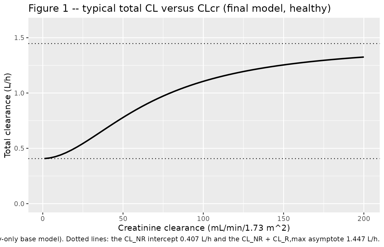
Figure 1 of Van Wart 2025 plots typical total clearance against CLcr. Note that the published curve comes from the base structural model fitted to healthy Phase 1 subjects only, whose parameter values are not reported; the final-model curve reproduced here is therefore comparable in shape and scale but not numerically identical. The published curve runs from about 0.37 L/h at CLcr = 0 to a plateau near 1.09 L/h.
cl is a variable in model(), so rxode2
returns it as an output column – the curve below is the packaged model’s
own arithmetic, not a re-implementation.
crcl_grid <- tibble(
  id = seq_len(60), CRCL = seq(1, 200, length.out = 60),
  arm = "typical healthy",
  WT = 79.7, AGE = 47.1, BMI = 27.3, SEXF = 0,
  DIS_HABP = 0, DIS_VABP = 0, DIS_BACTEREMIA = 0, DIS_CSSSI = 0,
  RRT_HEMODIAL_ACTIVE = 0, RRT_HEMODIAL_STATUS = 0, T_POST_HEMODIAL = 0,
  STUDY_TLV_PHASE2 = 0, STUDY_TLV_PHASE3 = 0
)

ev_crcl <- bind_rows(
  crcl_grid |> mutate(time = 0, evid = 1L, amt = 797, rate = -2,
                      cmt = "central", dvid = NA_integer_),
  crcl_grid |> mutate(time = 1, evid = 0L, amt = NA_real_, rate = NA_real_,
                      cmt = "central", dvid = 1L)
) |>
  arrange(id, time, desc(evid))

cl_curve <- solve_typical(ev_crcl, keep = c("CRCL")) |>
  filter(!is.na(cl)) |>
  group_by(CRCL) |>
  summarise(cl = mean(cl), .groups = "drop")
#> Warning: multi-subject simulation without without 'omega'

ggplot(cl_curve, aes(CRCL, cl)) +
  geom_line(linewidth = 0.9) +
  geom_hline(yintercept = 0.407, linetype = "dotted") +
  geom_hline(yintercept = 0.407 + 1.04, linetype = "dotted") +
  scale_y_continuous(limits = c(0, 1.6)) +
  labs(
    x = "Creatinine clearance (mL/min/1.73 m^2)",
    y = "Total clearance (L/h)",
    title = "Figure 1 -- typical total CL versus CLcr (final model, healthy)",
    caption = paste(
      "Replicates Figure 1 of Van Wart 2025 (which shows the healthy-only base",
      "model). Dotted lines: the CL_NR intercept 0.407 L/h and the",
      "CL_NR + CL_R,max asymptote 1.447 L/h."
    )
  )
cl_at <- function(x) cl_curve$cl[which.min(abs(cl_curve$CRCL - x))]

# The Hill function must be half-maximal in the renal arm at CLcr50 = 68.3.
cl_half <- cl_at(68.3)
stopifnot(abs(cl_half - (0.407 + 1.04 / 2)) < 0.01)

# Bracketed by the intercept and the asymptote everywhere.
stopifnot(all(cl_curve$cl > 0.407), all(cl_curve$cl < 0.407 + 1.04))

tibble::tibble(
  Quantity = c("CL at CLcr = 1", "CL at CLcr = 68.3 (CLcr50)",
               "CL at CLcr = 100", "CL at CLcr = 200"),
  `Model (L/h)` = round(c(cl_at(1), cl_half, cl_at(100), cl_at(200)), 3)
) |>
knitr::kable(caption = "Typical healthy total clearance at selected CLcr.")| Quantity | Model (L/h) |
|---|---|
| CL at CLcr = 1 | 0.407 |
| CL at CLcr = 68.3 (CLcr50) | 0.928 |
| CL at CLcr = 100 | 1.101 |
| CL at CLcr = 200 | 1.325 |
The half-maximal check is exact by construction of the Hill function
and confirms crcl50_cl_renal and hill_cl_renal
are wired into the renal arm rather than the total.
Figure 3 – plasma and ELF concentrations, 10 mg/kg q24h
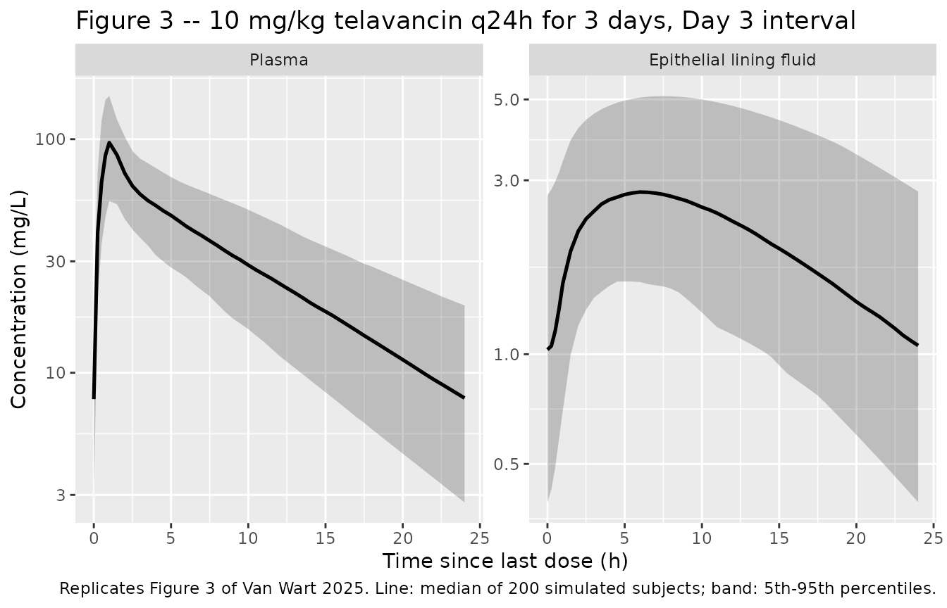
Figure 3 of Van Wart 2025 overlays a Monte Carlo simulation on the
observed Day 3 plasma and ELF data from Study I6424-108a. The published
median plasma curve peaks near 100 mg/L at the end of the 1-h infusion
and falls to roughly 2-3 mg/L at 24 h; the published median ELF curve
rises to a broad peak of about 2.7 mg/L between 4 and 8 h and declines
to about 1 mg/L by 24 h. The ELF peak is later and much flatter than the
plasma peak because k30 corresponds to a 4.5 h
half-life.
day3 <- sim_healthy |>
  filter(time >= 48) |>
  mutate(tsld = time - 48) |>
  select(id, tsld, Cc, Celf) |>
  pivot_longer(c(Cc, Celf), names_to = "matrix", values_to = "conc") |>
  mutate(matrix = factor(matrix, levels = c("Cc", "Celf"),
                         labels = c("Plasma", "Epithelial lining fluid")))

day3 |>
  group_by(matrix, tsld) |>
  summarise(
    Q05 = quantile(conc, 0.05, na.rm = TRUE),
    Q50 = quantile(conc, 0.50, na.rm = TRUE),
    Q95 = quantile(conc, 0.95, na.rm = TRUE),
    .groups = "drop"
  ) |>
  ggplot(aes(tsld, Q50)) +
  geom_ribbon(aes(ymin = Q05, ymax = Q95), alpha = 0.25) +
  geom_line(linewidth = 0.9) +
  facet_wrap(~matrix, scales = "free_y") +
  scale_y_log10() +
  labs(
    x = "Time since last dose (h)", y = "Concentration (mg/L)",
    title = "Figure 3 -- 10 mg/kg telavancin q24h for 3 days, Day 3 interval",
    caption = paste(
      "Replicates Figure 3 of Van Wart 2025. Line: median of", n_per_arm,
      "simulated subjects; band: 5th-95th percentiles."
    )
  )
peaks <- day3 |>
  group_by(matrix, tsld) |>
  summarise(Q50 = median(conc, na.rm = TRUE), .groups = "drop") |>
  group_by(matrix) |>
  summarise(
    peak_conc = max(Q50),
    peak_time = tsld[which.max(Q50)],
    at_24h    = Q50[which.min(abs(tsld - 24))],
    .groups   = "drop"
  )

peaks |>
  rename("Matrix" = matrix, "Median peak (mg/L)" = peak_conc,
         "Time of peak (h)" = peak_time, "Median at 24 h (mg/L)" = at_24h) |>
  knitr::kable(digits = 2, caption = paste(
    "Simulated Day 3 peak and 24-hour trough. Van Wart 2025 Figure 3 reads",
    "about 100 mg/L at 1 h for plasma and about 2.7 mg/L at 4-8 h for ELF,",
    "with observed 24-hour concentrations of roughly 5-14 mg/L (plasma) and",
    "0.6-2.4 mg/L (ELF)."
))| Matrix | Median peak (mg/L) | Time of peak (h) | Median at 24 h (mg/L) |
|---|---|---|---|
| Plasma | 96.69 | 1 | 7.79 |
| Epithelial lining fluid | 2.78 | 6 | 1.06 |
get_peak <- function(m, col) {
  v <- peaks[[col]][peaks$matrix == m]
  if (length(v) != 1L) stop("no unique peak row for '", m, "'")
  v
}

plasma_peak  <- get_peak("Plasma", "peak_conc")
plasma_24h   <- get_peak("Plasma", "at_24h")
elf_peak     <- get_peak("Epithelial lining fluid", "peak_conc")
elf_tmax     <- get_peak("Epithelial lining fluid", "peak_time")
elf_24h      <- get_peak("Epithelial lining fluid", "at_24h")

# Plasma peak within 30% of the ~100 mg/L read off Figure 3.
stopifnot(plasma_peak > 70, plasma_peak < 130)
# ELF peak within 30% of the ~2.7 mg/L read off Figure 3 ...
stopifnot(elf_peak > 1.9, elf_peak < 3.5)
# ... and, the qualitative signature of the biophase, much later than plasma.
stopifnot(elf_tmax >= 3)
# Both 24-hour troughs must land inside the observed ranges digitised from
# Figure 3. Note this is checked against the OBSERVED points, not against the
# paper's plotted median line -- see "Assumptions and deviations".
stopifnot(plasma_24h > 5, plasma_24h < 14)
stopifnot(elf_24h > 0.6, elf_24h < 2.4)
The plasma peak, the ELF peak, the ELF peak time and both 24-hour troughs land where Figure 3’s observed data sit. One caveat on the plasma trough is recorded in “Assumptions and deviations”: the simulated median at 24 h (about 8 mg/L) sits above the median line drawn in Figure 3 (about 2.5 mg/L), even though it sits squarely inside that figure’s own observed 24-hour concentrations.
PKNCA validation
Table 3 of Van Wart 2025 reports steady-state AUC0-24 in plasma and ELF, plus the ELF penetration ratios, for the 20 healthy subjects of Study I6424-108a. The NCA below is computed over the Day 3 dosing interval (48-72 h), which is the interval the paper sampled.
tau      <- 24
start_ss <- 48
end_ss   <- start_ss + tau

# Only !is.na() in the filter -- a `time > 0` or `Cc > 0` filter would drop the
# interval-anchoring record and trigger PKNCA's AUC-range warning.
sim_nca <- sim_healthy |>
  filter(!is.na(Cc), time >= start_ss, time <= end_ss) |>
  select(id, time, Cc, Celf, arm)

conc_obj <- PKNCA::PKNCAconc(
  as.data.frame(sim_nca), Cc ~ time | arm + id,
  concu = "mg/L", timeu = "h"
)

dose_df <- healthy |>
  filter(evid == 1, time == start_ss) |>
  select(id, time, amt, arm)

dose_obj <- PKNCA::PKNCAdose(
  as.data.frame(dose_df), amt ~ time | arm + id, doseu = "mg"
)

intervals <- data.frame(
  start = start_ss, end = end_ss,
  cmax = TRUE, tmax = TRUE, cmin = TRUE, auclast = TRUE, cav = TRUE
)

nca_plasma <- PKNCA::pk.nca(
  PKNCA::PKNCAdata(conc_obj, dose_obj, intervals = intervals)
)
The ELF endpoint gets its own PKNCA block, per the multi-output convention.
conc_obj_elf <- PKNCA::PKNCAconc(
  as.data.frame(sim_nca |> select(id, time, Celf, arm) |> rename(Cc = Celf)),
  Cc ~ time | arm + id, concu = "mg/L", timeu = "h"
)

nca_elf <- PKNCA::pk.nca(
  PKNCA::PKNCAdata(conc_obj_elf, dose_obj,
                   intervals = data.frame(start = start_ss, end = end_ss,
                                          cmax = TRUE, tmax = TRUE,
                                          auclast = TRUE, cav = TRUE))
)
Comparison against published NCA
published <- tibble::tribble(
  ~arm,                      ~auclast,
  "Healthy, 10 mg/kg q24h",  750
)

cmp_plasma <- nlmixr2lib::ncaComparisonTable(
  simulated     = nca_plasma,
  reference     = published,
  by            = "arm",
  units         = c(auclast = "mg*h/L", cmax = "mg/L", tmax = "h",
                    cmin = "mg/L", cav = "mg/L"),
  tolerance_pct = 20
)

knitr::kable(
  cmp_plasma,
  caption = paste(
    "Plasma steady-state NCA over the Day 3 interval versus Van Wart 2025",
    "Table 3 (plasma AUC0-24 mean 750 mg*h/L, median 757, range 570-954).",
    "* differs from reference by >20%. Rows with no published counterpart",
    "are reported for completeness."
  )
)| NCA parameter | arm | Reference | Simulated | % diff |
|---|---|---|---|---|
| AUClast (mg*h/L) | Healthy, 10 mg/kg q24h | 750 | 735 | -2.0% |
published_elf <- tibble::tribble(
  ~arm,                      ~auclast,
  "Healthy, 10 mg/kg q24h",  54.5
)

cmp_elf <- nlmixr2lib::ncaComparisonTable(
  simulated     = nca_elf,
  reference     = published_elf,
  by            = "arm",
  units         = c(auclast = "mg*h/L", cmax = "mg/L", tmax = "h",
                    cav = "mg/L"),
  tolerance_pct = 20
)

knitr::kable(
  cmp_elf,
  caption = paste(
    "ELF steady-state NCA over the Day 3 interval versus Van Wart 2025",
    "Table 3 (ELF AUC0-24 mean 54.5 mg*h/L, median 50.6, range 38.3-99.0).",
    "* differs from reference by >20%."
  )
)| NCA parameter | arm | Reference | Simulated | % diff |
|---|---|---|---|---|
| AUClast (mg*h/L) | Healthy, 10 mg/kg q24h | 54.5 | 48.6 | -10.9% |
ELF penetration ratio against the published values
auc_by_id <- function(res, name) {
  as.data.frame(res$result) |>
    filter(PPTESTCD == "auclast") |>
    select(id, !!name := PPORRES)
}

ratios <- auc_by_id(nca_plasma, "auc_plasma") |>
  inner_join(auc_by_id(nca_elf, "auc_elf"), by = "id") |>
  mutate(ratio_total = auc_elf / auc_plasma,
         ratio_free  = ratio_total / 0.10)  # 90% protein binding, Table 3 footnote d

stopifnot(nrow(ratios) == n_per_arm)

k13k30 <- 0.0107 / 0.154

elf_cmp <- tibble::tibble(
  Statistic = c("Total-drug ratio, median", "Total-drug ratio, mean",
                "Free-drug ratio, mean"),
  Simulated = c(median(ratios$ratio_total), mean(ratios$ratio_total),
                mean(ratios$ratio_free)),
  `Van Wart 2025 Table 3` = c(0.0683, 0.0730, 0.730)
) |>
  mutate(`% difference` = 100 * (Simulated - `Van Wart 2025 Table 3`) /
           `Van Wart 2025 Table 3`)

knitr::kable(elf_cmp, digits = 4, caption = paste(
  "ELF penetration ratio in the", n_per_arm, "subject cohort versus Van Wart",
  "2025 Table 3. The structural expectation is k13/k30 =",
  round(k13k30, 4), "; the cohort median sits slightly below it because k30",
  "carries IIV and the median of a 200-draw sample is noisy."
))| Statistic | Simulated | Van Wart 2025 Table 3 | % difference |
|---|---|---|---|
| Total-drug ratio, median | 0.0657 | 0.0683 | -3.7863 |
| Total-drug ratio, mean | 0.0724 | 0.0730 | -0.8711 |
| Free-drug ratio, mean | 0.7236 | 0.7300 | -0.8711 |
# Both published statistics must be reproduced within 10%.
stopifnot(abs(median(ratios$ratio_total) - 0.0683) / 0.0683 < 0.10)
stopifnot(abs(mean(ratios$ratio_total)   - 0.0730) / 0.0730 < 0.10)
Note that the exact structural identity
AUC_ELF / AUC_plasma = k13 / k30 is a property of the
typical-value model at true steady state, not of a finite sample:
k30 carries IIV (omega^2 = 0.113) while
k13 does not, so individual ratios are spread around
k13/k30 and a 200-subject median carries a few percent of
sampling noise. The identity itself is asserted to machine precision in
the next section. What this table shows is the separate and stronger
result that the cohort reproduces both published summary statistics.
Structural identities at steady state
Two identities pin the model’s arithmetic, and both are exact rather than approximate, so they are asserted tightly on a typical-value solve dosed to true steady state (20 days of q24h dosing, AUC integrated over the final interval):
- For a linear model the steady-state AUC over a dosing interval is
exactly
Dose / CL. This is a one-number check on the entire clearance sub-model – Hill function, weight and age powers, and infection shifts. - Integrating
dCelf/dt = k13*Cc - k30*Celfover a steady-state interval, theCelfincrement vanishes and every plasma parameter cancels, leavingAUC_ELF / AUC_plasma = k13 / k30exactly.
ident_subj <- tibble(
  id = 1:6, arm = "identity check",
  WT   = c(60, 79.7, 100, 79.7, 79.7, 120),
  AGE  = c(30, 47.1, 47.1, 75, 47.1, 47.1),
  BMI  = c(22, 27.3, 27.3, 27.3, 35, 27.3),
  CRCL = c(100, 100, 100, 100, 40, 100),
  SEXF = c(0, 0, 0, 0, 1, 1),
  DIS_HABP = 0, DIS_VABP = 0, DIS_BACTEREMIA = 0,
  DIS_CSSSI = c(0, 0, 1, 0, 1, 0),
  RRT_HEMODIAL_ACTIVE = 0, RRT_HEMODIAL_STATUS = 0, T_POST_HEMODIAL = 0,
  STUDY_TLV_PHASE2 = 0, STUDY_TLV_PHASE3 = 0
) |>
  mutate(dose_mg = 10 * WT)

ev_ident <- bind_rows(
  ident_subj |> crossing(time = seq(0, 480, by = 24)) |>
    mutate(evid = 1L, amt = dose_mg, rate = -2, cmt = "central",
           dvid = NA_integer_),
  ident_subj |> crossing(time = seq(480, 504, by = 0.05)) |>
    mutate(evid = 0L, amt = NA_real_, rate = NA_real_, cmt = "central",
           dvid = 1L)
) |>
  arrange(id, time, desc(evid))

sim_ident <- solve_typical(ev_ident, keep = c("WT", "CRCL", "arm"))
#> Warning: multi-subject simulation without without 'omega'

trapz <- function(x, y) sum(diff(x) * (head(y, -1) + tail(y, -1)) / 2)

ident <- sim_ident |>
  filter(!is.na(Cc), time >= 480) |>
  group_by(id, WT, CRCL) |>
  summarise(
    auc_sim  = trapz(time, Cc),
    auc_elf  = trapz(time, Celf),
    cl_model = mean(cl),
    .groups  = "drop"
  ) |>
  mutate(
    dose_mg      = 10 * WT,
    auc_pred     = dose_mg / cl_model,
    pct_diff     = 100 * (auc_sim - auc_pred) / auc_pred,
    elf_ratio    = auc_elf / auc_sim,
    elf_pct_diff = 100 * (elf_ratio - k13k30) / k13k30
  )

ident |>
  select(id, WT, CRCL, cl_model, auc_sim, auc_pred, pct_diff,
         elf_ratio, elf_pct_diff) |>
  rename("Subject" = id, "WT (kg)" = WT,
         "CLcr (mL/min/1.73 m^2)" = CRCL, "CL (L/h)" = cl_model,
         "AUC0-24,ss simulated (mg*h/L)" = auc_sim,
         "Dose / CL (mg*h/L)" = auc_pred, "% difference" = pct_diff,
         "ELF/plasma AUC ratio" = elf_ratio,
         "% difference vs k13/k30" = elf_pct_diff) |>
  knitr::kable(digits = 4, caption = paste(
    "Per-subject steady-state identities. Dosing for 20 days at 10 mg/kg",
    "q24h; AUC integrated over the final interval. Subjects vary in weight,",
    "age, BMI, sex, renal function and infection type, so both identities are",
    "tested across the whole covariate model."
))| Subject | WT (kg) | CLcr (mL/min/1.73 m^2) | CL (L/h) | AUC0-24,ss simulated (mg*h/L) | Dose / CL (mg*h/L) | % difference | ELF/plasma AUC ratio | % difference vs k13/k30 |
|---|---|---|---|---|---|---|---|---|
| 1 | 60.0 | 100 | 0.9121 | 657.8514 | 657.8513 | 0 | 0.0695 | 0 |
| 2 | 79.7 | 100 | 1.1058 | 720.7641 | 720.7640 | 0 | 0.0695 | 0 |
| 3 | 100.0 | 100 | 1.5321 | 652.6980 | 652.6979 | 0 | 0.0695 | 0 |
| 4 | 79.7 | 100 | 1.1542 | 690.5342 | 690.5342 | 0 | 0.0695 | 0 |
| 5 | 79.7 | 40 | 0.8418 | 946.7833 | 946.7832 | 0 | 0.0695 | 0 |
| 6 | 120.0 | 100 | 1.3747 | 872.9060 | 872.9059 | 0 | 0.0695 | 0 |
stopifnot(nrow(ident) == 6)
# Both identities are exact, so the tolerance is set at the numerical accuracy
# actually achieved (about 1e-5 %) rather than at a loose engineering margin.
stopifnot(max(abs(ident$pct_diff)) < 0.001)
stopifnot(max(abs(ident$elf_pct_diff)) < 0.001)
Both identities hold to better than 0.001% per subject – numerical-integration accuracy – across subjects that differ in weight, age, BMI, sex, renal function and infection type. The clearance sub-model and the ELF biophase are therefore internally consistent with the published parameter values.
The ELF identity is also what establishes that the ELF state holds a
concentration rather than an amount: had it been an
amount, the penetration ratio would additionally scale by
Vc / V_ELF, which would put it near 0.40 rather than 0.069,
and no ELF volume is reported anywhere in the paper or its
supplement.
Exposure across the populations of Figure 2
Figure 2 of Van Wart 2025 is a prediction-corrected VPC stratified by infection type and renal function; prediction correction removes the absolute scale, so the comparison here is on the direction and magnitude of the covariate effects rather than on a curve overlay. All arms receive 10 mg/kg q24h so the exposures are directly comparable.
arm_spec <- tibble::tribble(
  ~label,                        ~crcl, ~habp, ~vabp, ~bact, ~csssi, ~ph2, ~ph3,
  "Healthy, normal renal",         100,     0,     0,     0,      0,    0,    0,
  "cSSSI, normal renal",           100,     0,     0,     0,      1,    0,    1,
  "HABP/VABP, normal renal",       100,     1,     0,     0,      0,    0,    1,
  "cSSSI, moderate impairment",     45,     0,     0,     0,      1,    0,    1,
  "cSSSI, severe impairment",       20,     0,     0,     0,      1,    0,    1
)

set.seed(4131)
pops <- lapply(seq_len(nrow(arm_spec)), function(i) {
  s <- arm_spec[i, ]
  make_arm(
    n = n_per_arm, label = s$label, dose_mg_per_kg = 10,
    dose_times = c(0, 24, 48), obs_times = seq(48, 72, by = 0.25),
    wt_mean = 79.7, wt_sd = 21.5, age_mean = 47.1, age_sd = 18.4,
    bmi_mean = 27.3, bmi_sd = 6.99, crcl_mean = s$crcl,
    crcl_sd = max(5, s$crcl * 0.2), sexf_prob = 0.383,
    habp = s$habp, vabp = s$vabp, bacteremia = s$bact, csssi = s$csssi,
    phase2 = s$ph2, phase3 = s$ph3,
    id_offset = (i - 1L) * n_per_arm
  )
}) |>
  bind_rows()

stopifnot(!anyDuplicated(unique(pops[, c("id", "time", "evid")])))

sim_pops <- rxode2::rxSolve(
  mod, events = as.data.frame(pops), keep = keep_cols, useLinCmt = FALSE
) |>
  as.data.frame()

stopifnot(dplyr::n_distinct(sim_pops$id) == n_per_arm * nrow(arm_spec))

exposure <- sim_pops |>
  filter(!is.na(Cc), time >= 48) |>
  group_by(arm, id) |>
  summarise(auc = trapz(time, Cc), cmin = min(Cc), .groups = "drop") |>
  group_by(arm) |>
  summarise(
    `Median AUC0-24,ss (mg*h/L)` = median(auc),
    `5th-95th AUC` = sprintf("%.0f-%.0f", quantile(auc, 0.05), quantile(auc, 0.95)),
    `Median Cmin (mg/L)` = median(cmin),
    .groups = "drop"
  ) |>
  arrange(match(arm, arm_spec$label))

exposure |>
  rename("Population" = arm) |>
  knitr::kable(digits = 2, caption = paste(
    "Steady-state exposure by population, all at 10 mg/kg q24h.",
    n_per_arm, "subjects per arm."
))| Population | Median AUC0-24,ss (mg*h/L) | 5th-95th AUC | Median Cmin (mg/L) |
|---|---|---|---|
| Healthy, normal renal | 716.62 | 425-1155 | 8.66 |
| cSSSI, normal renal | 603.97 | 372-937 | 6.52 |
| HABP/VABP, normal renal | 512.03 | 307-867 | 6.09 |
| cSSSI, moderate impairment | 835.61 | 487-1420 | 13.89 |
| cSSSI, severe impairment | 1268.06 | 734-1912 | 27.14 |
# Look up by value, not by position, and fail loudly on a label mismatch: a
# lookup that quietly returns zero rows would make every stopifnot() below pass
# without testing anything.
get_med <- function(nm) {
  v <- exposure$`Median AUC0-24,ss (mg*h/L)`[exposure$arm == nm]
  if (length(v) != 1L) stop("no unique exposure row for '", nm, "'")
  v
}

stopifnot(all(arm_spec$label %in% exposure$arm))

# Infected patients have HIGHER clearance than healthy subjects (CL shifts are
# +0.418 and +0.228), so at the same dose their exposure must be LOWER.
stopifnot(get_med("cSSSI, normal renal")     < get_med("Healthy, normal renal"))
stopifnot(get_med("HABP/VABP, normal renal") < get_med("cSSSI, normal renal"))

# Renal impairment lowers clearance, so exposure must RISE as CLcr falls.
stopifnot(get_med("cSSSI, moderate impairment") > get_med("cSSSI, normal renal"))
stopifnot(get_med("cSSSI, severe impairment")   > get_med("cSSSI, moderate impairment"))
Both directions are as the model prescribes: the +0.418 and +0.228 clearance shifts make infected patients clear telavancin faster and so attain lower exposure at a given mg/kg dose, and falling CLcr moves down the Hill curve and raises exposure.
Intermittent hemodialysis
The dialysis structure is the part of the model with the fewest
supporting data (8 subjects) and two distinct time-varying covariates,
so it is exercised explicitly: RRT_HEMODIAL_ACTIVE gates
the +1.77 L/h dialysis clearance during each session, and
T_POST_HEMODIAL crossing 48 h switches on the +1.55 L
central-volume increase.
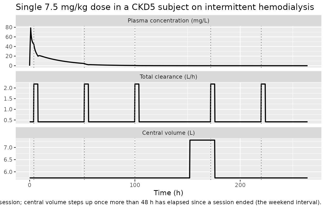
The regimen below is a single 7.5 mg/kg dose followed over ten days through a Monday/Wednesday/Friday schedule, chosen to mirror the single-dose renal- dysfunction studies in Table S1 and to include one weekend interval long enough to cross the 48-hour threshold. It is illustrative only and is not a dosing recommendation.
session_starts <- c(4, 52, 100, 172, 220)   # Mon/Wed/Fri, then next Mon/Wed
session_len    <- 4

ihd_grid <- tibble(time = seq(0, 264, by = 0.25)) |>
  rowwise() |>
  mutate(
    RRT_HEMODIAL_ACTIVE = as.integer(any(
      time >= session_starts & time < session_starts + session_len
    )),
    last_end = {
      ends <- session_starts + session_len
      done <- ends[ends <= time]
      if (length(done) == 0) NA_real_ else max(done)
    }
  ) |>
  ungroup() |>
  mutate(T_POST_HEMODIAL = ifelse(is.na(last_end), 0, time - last_end)) |>
  select(time, RRT_HEMODIAL_ACTIVE, T_POST_HEMODIAL)

ihd_cov <- tibble(
  id = 1L, arm = "CKD5 on IHD", WT = 79.7, AGE = 47.1, BMI = 27.3,
  CRCL = 5, SEXF = 0,
  DIS_HABP = 0, DIS_VABP = 0, DIS_BACTEREMIA = 0, DIS_CSSSI = 0,
  RRT_HEMODIAL_STATUS = 1,
  STUDY_TLV_PHASE2 = 0, STUDY_TLV_PHASE3 = 1
)

ev_ihd <- bind_rows(
  ihd_cov |>
    mutate(time = 0, evid = 1L, amt = 7.5 * 79.7, rate = -2,
           cmt = "central", dvid = NA_integer_,
           RRT_HEMODIAL_ACTIVE = 0, T_POST_HEMODIAL = 0),
  ihd_cov |>
    crossing(ihd_grid) |>
    mutate(evid = 0L, amt = NA_real_, rate = NA_real_, cmt = "central",
           dvid = 1L)
) |>
  arrange(time, desc(evid))

sim_ihd <- solve_typical(
  ev_ihd, keep = c("RRT_HEMODIAL_ACTIVE", "T_POST_HEMODIAL", "arm")
)

sim_ihd |>
  filter(!is.na(Cc)) |>
  select(time, Cc, cl_total, vc) |>
  pivot_longer(c(Cc, cl_total, vc)) |>
  mutate(name = factor(
    name, levels = c("Cc", "cl_total", "vc"),
    labels = c("Plasma concentration (mg/L)", "Total clearance (L/h)",
               "Central volume (L)")
  )) |>
  ggplot(aes(time, value)) +
  geom_line(linewidth = 0.8) +
  geom_vline(xintercept = session_starts, linetype = "dotted", colour = "grey40") +
  facet_wrap(~name, ncol = 1, scales = "free_y") +
  labs(
    x = "Time (h)", y = NULL,
    title = "Single 7.5 mg/kg dose in a CKD5 subject on intermittent hemodialysis",
    caption = paste(
      "Dotted lines mark the start of each 4-hour IHD session. Clearance steps",
      "up during each session; central volume steps up once more than 48 h has",
      "elapsed since a session ended (the weekend interval)."
    )
  )
ihd_obs <- sim_ihd |> filter(!is.na(Cc))

cl_on  <- unique(round(ihd_obs$cl_total[ihd_obs$RRT_HEMODIAL_ACTIVE == 1], 6))
cl_off <- unique(round(ihd_obs$cl_total[ihd_obs$RRT_HEMODIAL_ACTIVE == 0], 6))

stopifnot(length(cl_on) == 1L, length(cl_off) == 1L)

# The on/off difference must be exactly the published CL_DL of 1.77 L/h.
stopifnot(abs((cl_on - cl_off) - 1.77) < 1e-6)

vc_lo <- unique(round(ihd_obs$vc[ihd_obs$T_POST_HEMODIAL <= 48], 6))
vc_hi <- unique(round(ihd_obs$vc[ihd_obs$T_POST_HEMODIAL >  48], 6))

stopifnot(length(vc_lo) == 1L, length(vc_hi) == 1L)

# And the volume step must be exactly the published 1.55 L.
stopifnot(abs((vc_hi - vc_lo) - 1.55) < 1e-6)

tibble::tibble(
  Quantity = c("Total CL between sessions (L/h)", "Total CL during a session (L/h)",
               "Difference (published CL_DL = 1.77)",
               "Vc within 48 h of a session (L)", "Vc beyond 48 h (L)",
               "Difference (published 1.55 L)"),
  Value = c(cl_off, cl_on, cl_on - cl_off, vc_lo, vc_hi, vc_hi - vc_lo)
) |>
  knitr::kable(digits = 4, caption = paste(
    "Both dialysis covariate effects recovered exactly from the packaged model."
))| Quantity | Value |
|---|---|
| Total CL between sessions (L/h) | 0.4146 |
| Total CL during a session (L/h) | 2.1846 |
| Difference (published CL_DL = 1.77) | 1.7700 |
| Vc within 48 h of a session (L) | 5.7500 |
| Vc beyond 48 h (L) | 7.3000 |
| Difference (published 1.55 L) | 1.5500 |
Both dialysis effects are recovered to machine precision, which
confirms the RRT_HEMODIAL_ACTIVE and
T_POST_HEMODIAL gating is wired as published. The sawtooth
in total clearance and the single step in central volume are visible in
the figure above; note that with CRCL = 5 the
between-session clearance is almost entirely the 0.407 L/h non-renal
arm.
Assumptions and deviations
- Covariate normalization constants are not published. Van Wart 2025 prints no covariate equations and never states a reference weight, age or BMI. The model file normalizes each continuous covariate to its Table 1 population mean (TBW 79.7 kg, AGE 47.1 years, BMI 27.3 kg/m^2). See “Reference values for the covariate normalization” above for the three checks supporting this over both an uncentered model (falsified by roughly 15-fold on the absolute scale) and a rounded 70 kg reference (a poorer fit to Table 3 and to the labelled Vss). Any downstream user re-fitting this model should treat the reference values as a reconstruction, not a published quantity.
- The Table 2 CLd row label is corrupt. The weight exponent on distributional clearance is printed as “Vc-CLd-TBW power”. It is read here as the CLd-TBW power because it sits under the CLd heading, Vc already carries its own TBW power on a preceding row, Table S3 step 9 is “CLd / Weight / Power”, and the Abstract states that body weight was the only significant predictor of the variability in distributional clearance. The leading “Vc-” is a typesetting artifact carried down from the Vc rows.
- The sex effect on Vc is negative despite its row label. Table 2 labels the row “Vc-proportional increase for females” but reports -0.0584 with a 90% bootstrap CI of -0.0898 to -0.0293, entirely below zero. Females therefore have 5.84% lower central volume. The value and its interval are used as printed; the word “increase” in the label is not.
-
No typical infusion duration is reported. Table 2
gives
omega^2for D1 but no point estimate, because D1 came from recorded infusion start and stop times.lduris anchored at the paper’s documented default of 1 h (Methods, Data handling) and marked fixed, with the published IIV around it. Event tables must therefore userate = -2on dose rows so rxode2 takes the duration fromdur(central). - Study I6424-108a demographics are not published. The Figure 3 and Table 3 replications use the pooled Table 1 means for weight, age and BMI, with CLcr set to a nominal normal 100 mL/min/1.73 m^2. The paper states only that its own simulation used “the mean (standard deviation) of the subject covariate effects … from healthy subjects in Study I6424-108a” without printing them. A younger, higher-CLcr healthy cohort – the likely reality for a bronchoalveolar-lavage study – would shift the simulated plasma AUC0-24 by a few percent in either direction; this is the main source of the residual gap in the NCA comparison table.
-
The simulated 24-hour plasma trough exceeds the median line
drawn in Figure 3, but agrees with that figure’s own observed
data. The packaged model predicts a median Day 3 trough near 8
mg/L at 10 mg/kg q24h. Figure 3’s observed 24-hour concentrations run
from roughly 5 to 14 mg/L, so the prediction sits mid-range; but the
black median line in the same panel falls to about 2.5 mg/L, below every
observed point at that time. The discrepancy is therefore in the
published figure’s simulated line rather than in the extraction: the
steady-state AUC0-24 reproduces Table 3 to within 2%, the per-subject
AUC = Dose/CLidentity is exact, and a trough near 8 mg/L is what the pooled clearance and volume estimates imply. A plausible explanation is that the line was drawn from a single-dose rather than a Day 3 steady-state simulation, but the paper does not say, so this is left as an observation rather than a resolved error. Anyone using this model to predict troughs should weight Table 3 and the observed points over the plotted line. - Figure 1 is not numerically reproducible. The published curve comes from the base structural model fitted to Phase 1 healthy subjects only, and those parameter estimates are not reported. The reproduction above uses the final model and is comparable in shape and scale only.
-
Phase 2 and 3 residual magnitudes are reachable but unused
in most simulations.
STUDY_TLV_PHASE2andSTUDY_TLV_PHASE3select among the three published proportional residual terms. They affect only residual error, so they change thesimcolumn and notCc; the healthy arm sets both to 0 (the pooled Phase 1 / Phase 4 stratum), and the infected arms set the Phase 3 indicator. - The dialysis regimen shown is illustrative. The single 7.5 mg/kg dose and the Monday/Wednesday/Friday session schedule were chosen to exercise both time-varying dialysis covariates, including one interval long enough to cross the 48-hour threshold. Van Wart 2025 does not recommend a dialysis regimen, and neither does this vignette.
-
Race, height and BSA were screened but not
retained. They are recorded in the model file’s
covariatesDataExcludedmetadata rather thancovariateData, so the covariate screen’s provenance is preserved without declaring covariates the model never references. BSA still enters indirectly because CLcr is normalized to 1.73 m^2. -
The IIV on dialysis clearance is very imprecise.
omega^2for CL_DL is 0.0651 with a %SEM of 135 and a bootstrap 90% CI of 0.000944 to 0.129, reflecting the 8-subject base. It is encoded as published, but simulations that lean on between-subject variability in dialytic clearance should be treated as illustrative. - All parameter values come from the paper and its supplement. No value was taken from a figure, from author correspondence, or from an upstream model.