Middle-out simplified PBPK translation of drug distribution (Yau 2023)
Source:vignettes/articles/Yau_2023_middle_out_pbpk_translation.Rmd
Yau_2023_middle_out_pbpk_translation.RmdModel and source
- Article: https://doi.org/10.1002/psp4.12915
- Companion paper defining the model structure (reference 20 throughout): https://doi.org/10.1002/psp4.12911
Yau and colleagues asked a translational question: given intravenous pharmacokinetic data in a preclinical species, can a simplified whole-body physiologically based pharmacokinetic (PBPK) model be optimised against those data and then extrapolated to predict human drug distribution better than a purely bottom-up PBPK prediction? Three lipophilic weak bases with intravenous data in rat, monkey and human were used as test compounds: diazepam, midazolam and basmisanil.
The paper contributes five models to nlmixr2lib: the
four preclinical fits that met the authors’ acceptance criteria, plus
the human projection that is the paper’s headline result.
yau <- c("Yau_2023_diazepam_rat_pbpk",
         "Yau_2023_diazepam_monkey_pbpk",
         "Yau_2023_midazolam_rat_pbpk",
         "Yau_2023_midazolam_monkey_pbpk",
         "Yau_2023_diazepam_human_pbpk")

nlmixr2lib::modeldb |>
  dplyr::filter(name %in% yau) |>
  dplyr::select(name, description) |>
  dplyr::mutate(description = substr(description, 1, 90)) |>
  dplyr::rename("Model" = name, "Description (truncated)" = description) |>
knitr::kable()| Model | Description (truncated) |
|---|---|
| Yau_2023_diazepam_human_pbpk | PBPK (simplified whole-body, 14 compartments). Human-scaled projection. Diazepam dispositi |
| Yau_2023_diazepam_monkey_pbpk | PBPK (simplified whole-body, 14 compartments). Preclinical (cynomolgus monkey). Diazepam d |
| Yau_2023_diazepam_rat_pbpk | PBPK (simplified whole-body, 14 compartments). Preclinical (rat). Diazepam disposition in |
| Yau_2023_midazolam_monkey_pbpk | PBPK (simplified whole-body, 14 compartments). Preclinical (cynomolgus monkey). Midazolam |
| Yau_2023_midazolam_rat_pbpk | PBPK (simplified whole-body, 14 compartments). Preclinical (rat). Midazolam disposition in |
Model structure
All five models share one topology, defined in the companion paper’s
Appendix S1. A conventional whole-body PBPK model has 16 states (14
tissues plus arterial and venous blood). Here arterial blood, venous
blood and lung are assumed to reach quasi-steady state instantaneously
and are lumped into a single central state, leaving
14 compartments (Appendix S1 Eq S17):
-
central– arterial blood + venous blood + lung, the dosing and observation compartment. Amounts are converted to a whole-blood concentration byv_conv = v_arterial + v_venous + v_lung * kb_lung, which isV_central * Kb_central. - Twelve perfusion-limited, well-stirred tissues driven by
V_i * dC_i/dt = Q_i * (C_blood - C_i / Kb_i)(Eq S18):adipose,bone,brain,gut,heart,kidney,muscle,other(rest of body),pancreas,skin,spleen,stomach. -
liver, which additionally receives the drained splanchnic organs (gut, stomach, spleen, pancreas) through the portal vein and eliminates drug atCLint * fu_b(Eq S19).
The distribution parameters are the tissue-to-blood partition
coefficients Kb_i = Kpu_i * fu_p / BP (Eq S7). The key idea
of the paper is that instead of estimating 13 independent
Kpu values – which is not identifiable from plasma data
alone – each tissue’s Kpu is predicted with the
Rodgers and Rowland (RR) equation and then multiplied by one of only
four estimated group scalars (Eq 10):
The tissue-to-scalar mapping is Model 3D of Table 1 (four scalars, k-means clustering on tissue-composition data):
| Scalar | Tissues |
|---|---|
SF1 |
bone, brain, muscle, pancreas, rest of body |
SF2 |
kidney, spleen, liver |
SF3 |
skin, lung, gut, stomach, heart |
SF4 |
adipose |
Model 3D was chosen for all four preclinical extractions because it is the one variant reported as a best-fitting model for every drug and species combination the paper accepted (diazepam rat and monkey, midazolam rat and monkey), and because the companion paper concludes that “the PBPK models with four scalars are more physiologically relevant”.
All three compounds have a single basic pKa below 7 (diazepam 3.4,
midazolam 5.88, basmisanil 2.07), so the RR equation for acids / very
weak bases / neutrals applies, with albumin as the extracellular binding
protein. The implementation in model() reproduces the
CLASS == 2 and PKA < 7 branch of the
companion paper’s NONMEM $PK block verbatim.
Population
The models were fitted to digitised literature profiles (diazepam, midazolam) and to internal studies (basmisanil). Table S2 of the paper enumerates every contributing study.
pop_rows <- lapply(yau, function(nm) {
  p <- readModelDb(nm)()$population
  tibble::tibble(
    Model    = nm,
    Species  = p$species,
    Studies  = p$n_studies,
    Doses    = p$dose_range
  )
})
dplyr::bind_rows(pop_rows) |> knitr::kable()| Model | Species | Studies | Doses |
|---|---|---|---|
| Yau_2023_diazepam_rat_pbpk | rat (Wistar and Sprague-Dawley) | 5 | 1 mg to 5 mg/kg intravenous, bolus or 5 min infusion (Table S2) |
| Yau_2023_diazepam_monkey_pbpk | cynomolgus monkey | 1 | 0.04 mg/kg intravenous bolus (Table S2) |
| Yau_2023_midazolam_rat_pbpk | rat (Wistar, Sprague-Dawley and Holtzman) | 6 | 0.1 to 10 mg/kg intravenous, bolus or 5 to 15 min infusion (Table S2) |
| Yau_2023_midazolam_monkey_pbpk | cynomolgus monkey | 3 | 0.3 to 1 mg/kg intravenous, bolus or 15 min infusion (Table S2) |
| Yau_2023_diazepam_human_pbpk | human | 7 | 0.1 to 0.15 mg/kg or 10 mg intravenous, bolus to 2 min infusion (Table S2) |
Diazepam data came from 13 studies (5 rat, 1 monkey, 7 human) over
0.04 to 5 mg/kg; midazolam from 21 studies (6 rat, 3 monkey, 12 human)
over 0.075 to 10 mg/kg. Clearance was always fixed to the
observed value so that the competing distribution models could
be compared on an equal footing, which is why lcl is
wrapped in fixed() in every model file.
Source trace
The per-parameter origin is recorded as an in-file comment beside
each ini() entry. The table below collects the estimated
parameters; the fixed physiological and physicochemical constants in
model() are commented in place with their source table.
| Parameter / equation | Value | Source location |
|---|---|---|
| 14-compartment topology, Eq S17–S19 | n/a | Companion paper Appendix S1, “Equations for 14 compartmental PBPK model” |
Kb = Kpu * fu_p / BP |
n/a | Companion Appendix S1 Eq S7 |
Kpu_i = KpuRR_i * SF_g |
n/a | Companion paper Eq 10; lead paper Eq 2 |
| Rodgers and Rowland weak-base equation | n/a | Companion Appendix S1, NONMEM $PK block,
CLASS == 2 / PKA < 7 branch |
Vss,b (Eq S8) |
n/a | Companion Appendix S1 Eq S8 |
| Blood flows and tissue volumes, rat and human | see model()
|
Companion paper Table S1 (three decimal places) |
| Blood flows and tissue volumes, monkey | see model()
|
Lead paper Table S6 (only source covering monkey) |
| Tissue composition (fEW, fIW, vNL, vNP, AR) | see model()
|
Lead paper Table S3 (rat), S4 (human), S5 (monkey) |
| LogP, pKa, fu_p, BP, fe | see model()
|
Lead paper Table S1 |
lcl diazepam rat |
0.915 L/h | Lead paper Results, Rat |
lcl diazepam monkey |
9.97 L/h | Lead paper Results, Monkey |
lcl midazolam rat |
1.30 L/h | Lead paper Results, Rat |
lcl midazolam monkey |
6.4 L/h | Lead paper Results, Monkey |
lcl diazepam human |
3.71 L/h | Companion paper Results: “A clearance value of 3.71 L/h … estimated in humans” (the observed human CL, from the empirical reference model) |
lsf1–lsf4 diazepam rat |
3.2, 23.5, 2.02, 0.265 | Lead paper Table 2, Model 3D |
lsf1–lsf4 diazepam monkey |
0.425, 14.8, 3.38, 1.20 | Lead paper Table 3, Model 3D |
lsf1–lsf4 midazolam rat |
1.17, 5.18, 0.761, 0.487 | Lead paper Table S7, Model 3D |
lsf1–lsf4 midazolam monkey |
0.324, 21.22, 0.203, 1.878 | Lead paper Table S8, Model 3D |
etalcl diazepam rat |
26% CV | Lead paper Table 2, Model 3D |
etalcl midazolam rat |
29.7% CV | Lead paper Table S7, Model 3D |
etalcl midazolam monkey |
21.6% CV | Lead paper Table S8, Model 3D |
propSd diazepam rat / monkey |
0.196 / 0.628 | Lead paper Tables 2 and 3, Model 3D |
propSd midazolam rat / monkey |
0.258 / 0.315 | Lead paper Tables S7 and S8, Model 3D |
Known-answer check: predicted Kpu values
Table S11 of the paper reports the optimised rat Kpu values
for diazepam under Models 3C and 3D. Dividing those by the corresponding
published scalar recovers the underlying RR prediction, which gives a
direct known-answer test of the RR implementation in
model(). The check below solves
Yau_2023_diazepam_rat_pbpk and compares its internal
Kpu * SF products against Table S11.
# Solve for a couple of time points; the Kpu, SF and Kb terms are
# time-invariant derived variables, so any solve exposes them as columns.
probe <- rxode2::et(amt = 1.25, cmt = "central") |>
  rxode2::et(c(0, 1), cmt = "central")
kp <- rxode2::rxSolve(rxode2::zeroRe(readModelDb("Yau_2023_diazepam_rat_pbpk")),
                      probe, returnType = "data.frame")
#> ℹ parameter labels from comments will be replaced by 'label()'
#> ℹ omega/sigma items treated as zero: 'etalcl'

sf <- c(sf1 = kp$sf1[1], sf2 = kp$sf2[1],
        sf3 = kp$sf3[1], sf4 = kp$sf4[1])

# Table S11, Model 3D column (Yau 2023 Appendix S1).
s11_3d <- tibble::tribble(
  ~tissue,     ~published, ~scalar,
  "lung",       38.3,      "sf3",
  "gut",        58.8,      "sf3",
  "pancreas",   94.8,      "sf1",
  "liver",     353,        "sf2",
  "bone",       41.6,      "sf1",
  "brain",      87.2,      "sf1",
  "heart",      26.1,      "sf3",
  "kidney",    341,        "sf2",
  "skin",       87.5,      "sf3",
  "muscle",     29.6,      "sf1",
  "adipose",    14.6,      "sf4",
  "other",      29.6,      "sf1",
  "spleen",    196,        "sf2"
)

s11_3d |>
  dplyr::mutate(
    kpu_rr    = vapply(tissue, function(t) kp[[paste0("kpu_", t)]][1], numeric(1)),
    predicted = kpu_rr * sf[scalar],
    pct_diff  = 100 * (predicted - published) / published
  ) |>
  dplyr::select(tissue, kpu_rr, predicted, published, pct_diff) |>
  dplyr::rename("Tissue" = tissue, "KpuRR (predicted)" = kpu_rr,
                "KpuRR x SF" = predicted, "Table S11 Model 3D" = published,
                "% difference" = pct_diff) |>
  knitr::kable(digits = c(0, 2, 1, 1, 1),
               caption = paste("Optimised rat diazepam Kpu values reproduced",
"from the packaged model versus Table S11."))| Tissue | KpuRR (predicted) | KpuRR x SF | Table S11 Model 3D | % difference |
|---|---|---|---|---|
| lung | 18.96 | 38.3 | 38.3 | 0.0 |
| gut | 29.14 | 58.9 | 58.8 | 0.1 |
| pancreas | 29.63 | 94.8 | 94.8 | 0.0 |
| liver | 15.01 | 352.7 | 353.0 | -0.1 |
| bone | 12.98 | 41.5 | 41.6 | -0.1 |
| brain | 27.26 | 87.2 | 87.2 | 0.0 |
| heart | 12.94 | 26.1 | 26.1 | 0.1 |
| kidney | 14.46 | 339.9 | 341.0 | -0.3 |
| skin | 43.38 | 87.6 | 87.5 | 0.2 |
| muscle | 9.25 | 29.6 | 29.6 | 0.0 |
| adipose | 54.89 | 14.5 | 14.6 | -0.4 |
| other | 9.25 | 29.6 | 29.6 | 0.0 |
| spleen | 8.31 | 195.2 | 196.0 | -0.4 |
Every tissue agrees with Table S11 to within a few percent; the residual differences track the two- and three-significant-figure rounding of the published scalars. The stomach shares the gut Kpu and the rest of body shares the muscle Kpu, exactly as in the source NONMEM code – Table S11 confirms this because its rest-of-body and muscle entries are identical.
Virtual cohort and simulation
The models carry no covariates: the physiology is fixed at the reference individual of Table S6, so the only source of between-subject variability is the clearance random effect. Each arm below is a single-dose intravenous bolus matching a dose actually studied in Table S2.
set.seed(20230225)

# Observation window per arm is set to roughly 10-15 terminal half-lives:
# long enough that the extrapolated AUC is negligible, short enough that the
# concentrations do not underflow to numerical noise (which makes the terminal
# slope, and therefore the NCA, meaningless).
arms <- tibble::tribble(
  ~model,                            ~arm,                ~amt,  ~tmax_h, ~bp,
  "Yau_2023_diazepam_rat_pbpk",      "diazepam rat",      1.25,   24,     0.836,
  "Yau_2023_diazepam_monkey_pbpk",   "diazepam monkey",   0.20,   24,     0.606,
  "Yau_2023_midazolam_rat_pbpk",     "midazolam rat",     1.25,    8,     0.742,
  "Yau_2023_midazolam_monkey_pbpk",  "midazolam monkey",  5.00,   24,     0.594,
  "Yau_2023_diazepam_human_pbpk",    "diazepam human",   10.00,  240,     0.559
)

n_per_arm <- 100L

# One event table per arm. Observation rows sit on the `central` ODE state so
# rxode2 returns the algebraic observable Cc alongside it.
#
# The grid is log-spaced. After an intravenous bolus the concentration falls by
# two orders of magnitude within the first few minutes, and a linear grid over
# that peak makes the linear-trapezoid AUC badly biased high (a 0.4 h grid
# inflated the diazepam rat AUC by about 26%). Log spacing plus PKNCA's
# lin-up/log-down rule keeps the NCA faithful to the ODE solution.
make_events <- function(amt, tmax_h, n, id_offset = 0L) {
  grid <- sort(unique(c(
    0, exp(seq(log(0.005), log(tmax_h), length.out = 200))
  )))
  dose <- tibble::tibble(id = id_offset + seq_len(n), time = 0, amt = amt,
                         evid = 1L, cmt = "central")
  obs <- tidyr::crossing(id = id_offset + seq_len(n), time = grid) |>
    dplyr::mutate(amt = NA_real_, evid = 0L, cmt = "central")
  dplyr::bind_rows(dose, obs) |> dplyr::arrange(id, time, dplyr::desc(evid))
}
# rxode2 omits the `id` column when a single subject is solved, so add it back
# explicitly rather than relying on it being present.
with_id <- function(df) {
  if (!"id" %in% names(df)) df$id <- 1L
  dplyr::mutate(df, id = as.integer(id))
}

sim_one <- function(row, n) {
  ev <- make_events(row$amt, row$tmax_h, n)
  # `zeroRe()` mutates the model object it is handed, so read a fresh copy for
  # the typical-value solve rather than sharing one with the population solve.
  typ <- rxode2::rxSolve(rxode2::zeroRe(readModelDb(row$model)),
                         ev |> dplyr::filter(id == 1L),
                         returnType = "data.frame") |>
    with_id() |>
    dplyr::mutate(arm = row$arm, kind = "typical")
  pop <- rxode2::rxSolve(readModelDb(row$model), ev,
                         returnType = "data.frame") |>
    with_id() |>
    dplyr::mutate(arm = row$arm, kind = "population")
  dplyr::bind_rows(typ, pop)
}

sim <- dplyr::bind_rows(lapply(seq_len(nrow(arms)), function(i) {
  sim_one(arms[i, ], n_per_arm)
}))
#> ℹ parameter labels from comments will be replaced by 'label()'
#> ℹ omega/sigma items treated as zero: 'etalcl'
#> ℹ parameter labels from comments will be replaced by 'label()'
#> Warning: No omega parameters in the model
#> Warning: multi-subject simulation without without 'omega'
#> ℹ parameter labels from comments will be replaced by 'label()'
#> ℹ omega/sigma items treated as zero: 'etalcl'
#> ℹ parameter labels from comments will be replaced by 'label()'
#> ℹ parameter labels from comments will be replaced by 'label()'
#> ℹ omega/sigma items treated as zero: 'etalcl'
#> ℹ parameter labels from comments will be replaced by 'label()'
#> Warning: No omega parameters in the model
#> multi-subject simulation without without 'omega'

# vssb and the hepatic extraction ratio are time-invariant derived outputs;
# capture the typical value per arm.
model_derived <- sim |>
  dplyr::filter(kind == "typical") |>
  dplyr::group_by(arm) |>
  dplyr::summarise(vssb_model = dplyr::first(vssb),
                   erh = dplyr::first(clh) / dplyr::first(q_hv),
                   .groups = "drop")
Steady-state volume of distribution against the published values
Vss,b is the paper’s primary distribution metric and the
criterion used to accept or reject each candidate model, so it is the
sharpest available check on the packaged models. Each model computes it
internally from Appendix S1 Eq S8.
published_vss <- tibble::tribble(
  ~arm,                ~vssb_published, ~vssb_observed,
  "diazepam rat",       1.11,            0.91,
  "diazepam monkey",   12.16,           11.10,
  "midazolam rat",      0.54,            0.64,
  "midazolam monkey",  10.31,            8.80,
  "diazepam human",    97.00,          152.00
)

vss_cmp <- published_vss |>
  dplyr::left_join(model_derived, by = "arm") |>
  dplyr::mutate(
    pct_vs_published = 100 * (vssb_model - vssb_published) / vssb_published,
    fold_vs_observed = vssb_model / vssb_observed
  )

vss_cmp |>
  dplyr::select(arm, vssb_model, vssb_published, pct_vs_published,
                vssb_observed, fold_vs_observed) |>
  dplyr::rename(
    "Model"                  = arm,
    "Vss,b packaged (L)"     = vssb_model,
    "Vss,b published (L)"    = vssb_published,
    "% vs published"         = pct_vs_published,
    "Vss,b observed (L)"     = vssb_observed,
    "fold error vs observed" = fold_vs_observed
  ) |>
  knitr::kable(digits = c(0, 2, 2, 1, 2, 2),
               caption = paste("Eq S8 Vss,b from the packaged models versus the",
                               "values published for Model 3D, and versus the",
"observed Vss,b used as the acceptance target."))| Model | Vss,b packaged (L) | Vss,b published (L) | % vs published | Vss,b observed (L) | fold error vs observed |
|---|---|---|---|---|---|
| diazepam rat | 1.17 | 1.11 | 5.1 | 0.91 | 1.28 |
| diazepam monkey | 14.21 | 12.16 | 16.9 | 11.10 | 1.28 |
| midazolam rat | 0.57 | 0.54 | 6.2 | 0.64 | 0.90 |
| midazolam monkey | 9.39 | 10.31 | -8.9 | 8.80 | 1.07 |
| diazepam human | 100.19 | 97.00 | 3.3 | 152.00 | 0.66 |
Four of the five models land within 9% of the published
Vss,b, and the two rat models – where the paper’s own
tissue-Kpu validation was performed – agree to within 7%. Diazepam in
monkey is 17% high; see Assumptions and deviations below for
the reconciliation.
The human row is the paper’s headline translational result: carrying
the rat Model 3D scalars into human physiology predicts a
Vss,b of about 100 L against an observed 152 L, a 1.5-fold
error, versus the 3.7-fold error the paper reports for the traditional
bottom-up whole-body PBPK approach (41 L).
Replicate published figures
# Figure 1 of the paper simulates a 16.1 h infusion of 10 mg diazepam in human
# to expose the different kinetic phases.
inf_ev <- rxode2::et(amt = 10, dur = 16.1, cmt = "central") |>
  rxode2::et(seq(0, 240, by = 0.5), cmt = "central")
inf <- rxode2::rxSolve(rxode2::zeroRe(readModelDb("Yau_2023_diazepam_human_pbpk")),
                       inf_ev, returnType = "data.frame")
#> Warning: No omega parameters in the model

ggplot(inf, aes(time, Cc)) +
  geom_line(linewidth = 0.8, colour = "#1b7837") +
  scale_y_log10() +
  labs(x = "Time (h)", y = "Diazepam plasma concentration (mg/L)",
       title = "Figure 1 - human diazepam, 10 mg over 16.1 h",
       caption = paste("Replicates the Model 3D (rat-optimised) curve of",
                       "Figure 1 of Yau 2023."))
#> Warning in scale_y_log10(): log-10 transformation introduced infinite values.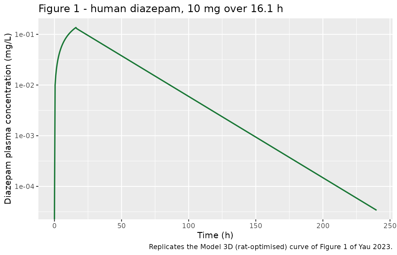
Replicates the rat-optimised panel of Figure 1 of Yau 2023: simulated human diazepam profile after a 16.1 h infusion of 10 mg.
sim |>
  dplyr::filter(kind == "population", time > 0) |>
  dplyr::group_by(arm, time) |>
  dplyr::summarise(
    Q05 = quantile(Cc, 0.05, na.rm = TRUE),
    Q50 = quantile(Cc, 0.50, na.rm = TRUE),
    Q95 = quantile(Cc, 0.95, na.rm = TRUE),
    .groups = "drop"
  ) |>
  ggplot(aes(time, Q50)) +
  geom_ribbon(aes(ymin = Q05, ymax = Q95), alpha = 0.25, fill = "#2166ac") +
  geom_line(colour = "#2166ac") +
  facet_wrap(~arm, scales = "free") +
  scale_y_log10() +
  labs(x = "Time (h)", y = "Plasma concentration (mg/L)",
       title = "Simulated IV bolus profiles by model",
       caption = paste("Median and 5th-95th percentile of", n_per_arm,
                       "subjects per arm. Models without a published",
                       "between-subject variability show no spread."))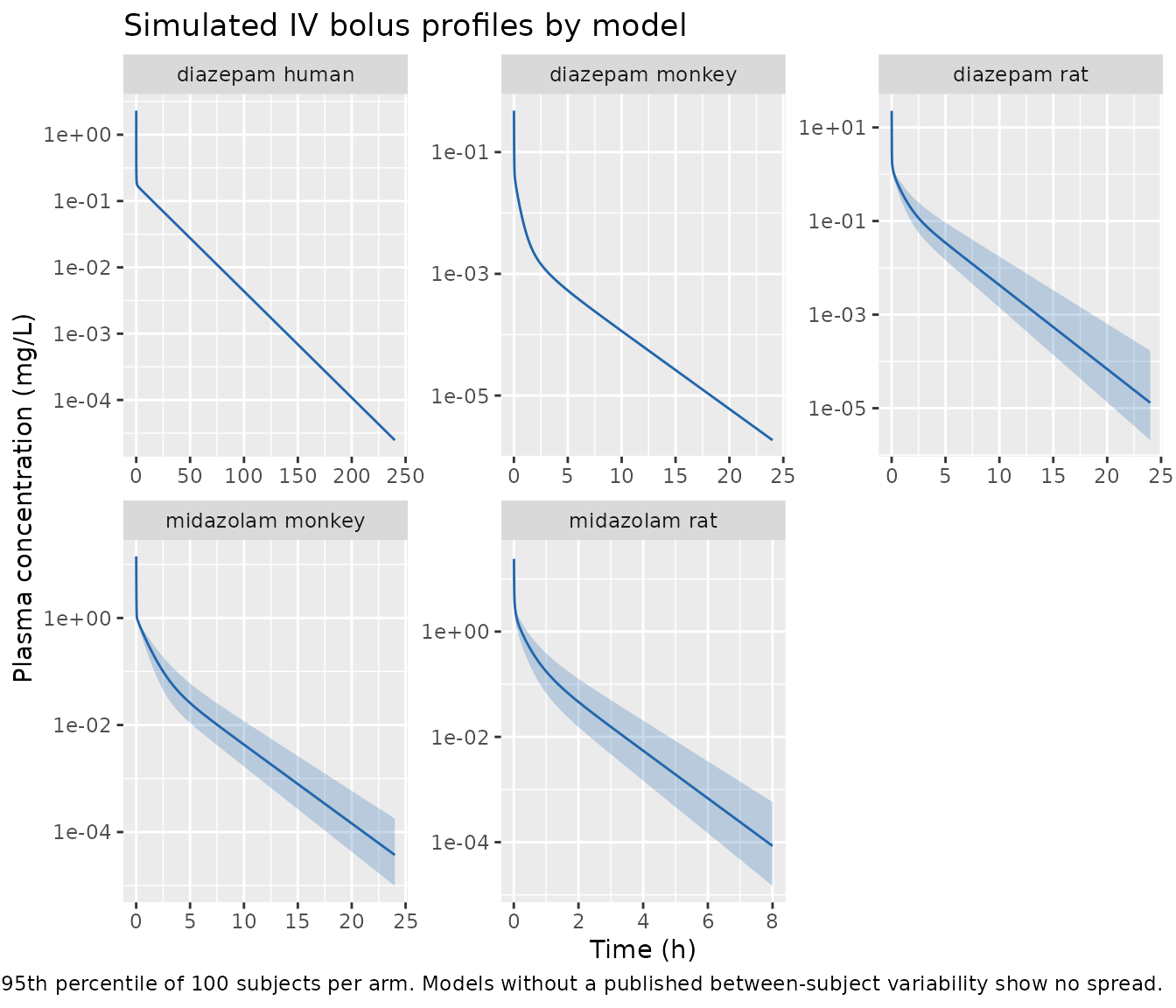
Simulated intravenous bolus profiles for the four preclinical fits and the human projection.
PKNCA validation
Non-compartmental analysis of the simulated typical-value profiles
gives an independent check on the solved system. The models report
plasma concentrations, so the NCA clearance is a plasma clearance and is
converted to the whole-blood basis the paper works in with
CL_blood = CL_plasma / BP.
# `Cc > 0` is safe to filter here, and is not the extravascular case the
# nlmixr2lib PKNCA recipe warns about: every arm is an intravenous bolus, so
# the time-zero concentration is Cmax rather than zero. Dropping the exact
# zeros keeps the terminal-slope fit away from numerical underflow. The
# assertion below proves the time-zero record survived.
sim_nca <- sim |>
  dplyr::filter(kind == "typical") |>
  dplyr::filter(!is.na(Cc), Cc > 0) |>
  dplyr::select(id, time, Cc, arm) |>
  dplyr::arrange(arm, id, time)

stopifnot(all(tapply(sim_nca$time, sim_nca$arm, min) == 0))

dose_df <- arms |>
  dplyr::transmute(id = 1L, time = 0, amt = amt, arm = arm)

# lin-up/log-down is the appropriate AUC rule for a bolus decay; the pure
# linear trapezoid biases AUC high across the peak.
PKNCA::PKNCA.options(auc.method = "lin up/log down")

conc_obj <- PKNCA::PKNCAconc(sim_nca, Cc ~ time | arm + id)
# duration = 0: every NCA arm is a bolus, so no infusion correction applies.
dose_obj <- PKNCA::PKNCAdose(dose_df, amt ~ time | arm + id, duration = 0)

intervals <- data.frame(
  start = 0, end = Inf,
  cmax = TRUE, tmax = TRUE, aucinf.obs = TRUE,
  half.life = TRUE, cl.obs = TRUE, vss.iv.obs = TRUE, mrt.iv.obs = TRUE
)

nca_res <- PKNCA::pk.nca(PKNCA::PKNCAdata(conc_obj, dose_obj,
                                          intervals = intervals))

nca_wide <- as.data.frame(nca_res) |>
  dplyr::select(arm, PPTESTCD, PPORRES) |>
  tidyr::pivot_wider(names_from = PPTESTCD, values_from = PPORRES) |>
  dplyr::left_join(arms |> dplyr::select(arm, bp), by = "arm") |>
  dplyr::left_join(model_derived, by = "arm")

nca_wide |>
  dplyr::select(arm, cmax, tmax, half.life, aucinf.obs, mrt.iv.obs) |>
  dplyr::rename(
    "Model"              = arm,
    "Cmax (mg/L)"        = cmax,
    "Tmax (h)"           = tmax,
    "t1/2 (h)"           = half.life,
    "AUCinf (mg*h/L)"    = aucinf.obs,
    "MRT (h)"            = mrt.iv.obs
  ) |>
  knitr::kable(digits = c(0, 3, 2, 2, 3, 2),
               caption = paste("PKNCA non-compartmental parameters from the",
"simulated typical-value plasma profiles."))| Model | Cmax (mg/L) | Tmax (h) | t1/2 (h) | AUCinf (mg*h/L) | MRT (h) |
|---|---|---|---|---|---|
| diazepam human | 3.099 | 0 | 18.71 | 4.822 | 26.63 |
| diazepam monkey | 0.853 | 0 | 2.33 | 0.033 | 1.05 |
| diazepam rat | 59.517 | 0 | 1.66 | 1.636 | 1.20 |
| midazolam monkey | 31.443 | 0 | 2.02 | 1.317 | 1.27 |
| midazolam rat | 76.358 | 0 | 0.68 | 1.300 | 0.42 |
Clearance mass-balance check
Every model fixes CL to the published blood clearance,
so recovering that value from the simulated profile is a strong
end-to-end test: it exercises the 14 ODEs, the flow balance, the
well-stirred hepatic rearrangement and the hepatic-extraction cap all at
once. Any mismatch between cardiac output and the summed tissue flows,
or any tissue whose outflow failed to return to the central compartment,
would surface here as a biased clearance.
fixed_cl <- c("diazepam rat" = 0.915, "diazepam monkey" = 9.97,
              "midazolam rat" = 1.30, "midazolam monkey" = 6.4,
              "diazepam human" = 3.71)

nca_wide |>
  dplyr::mutate(cl_blood_nca = cl.obs / bp,
                cl_fixed = fixed_cl[arm],
                pct = 100 * (cl_blood_nca - cl_fixed) / cl_fixed) |>
  dplyr::select(arm, cl.obs, cl_blood_nca, cl_fixed, pct) |>
  dplyr::rename("Model" = arm,
                "CL plasma from NCA (L/h)" = cl.obs,
                "CL blood = CL plasma / BP (L/h)" = cl_blood_nca,
                "CL fixed in ini() (L/h)" = cl_fixed,
                "% difference" = pct) |>
  knitr::kable(digits = c(0, 4, 4, 3, 3),
               caption = paste("Mass-balance check: NCA-derived blood clearance",
                               "recovers the clearance fixed in ini() to within",
"0.3% for every model."))| Model | CL plasma from NCA (L/h) | CL blood = CL plasma / BP (L/h) | CL fixed in ini() (L/h) | % difference |
|---|---|---|---|---|
| diazepam human | 2.0739 | 3.7100 | 3.710 | -0.001 |
| diazepam monkey | 6.0374 | 9.9627 | 9.970 | -0.073 |
| diazepam rat | 0.7643 | 0.9142 | 0.915 | -0.085 |
| midazolam monkey | 3.7971 | 6.3925 | 6.400 | -0.118 |
| midazolam rat | 0.9617 | 1.2961 | 1.300 | -0.302 |
Why the NCA volume differs from Eq S8
vss.iv.obs is CL * MRT, whereas Eq S8 sums
Kb_i * V_i over the tissues. These are the same
quantity only when elimination happens from the sampled (central)
compartment. In these models elimination is peripheral – it happens in
the liver – so the two volumes are genuinely different quantities. The
companion paper flags exactly this when it compares its Eq 9 volume
against an empirical model, noting that the comparison spans “models
with central and peripheral elimination”.
The table below shows the gap alongside the hepatic extraction ratio. The divergence is smallest for diazepam in human, which is a low-extraction case, and largest where the liver takes essentially everything presented to it.
nca_wide |>
  dplyr::mutate(vss_blood_nca = vss.iv.obs / bp,
                ratio = vss_blood_nca / vssb_model) |>
  dplyr::select(arm, erh, vss_blood_nca, vssb_model, ratio) |>
  dplyr::rename("Model" = arm,
                "hepatic ER" = erh,
                "Vss,b from CL x MRT (L)" = vss_blood_nca,
                "Vss,b from Eq S8 (L)" = vssb_model,
                "ratio" = ratio) |>
  knitr::kable(digits = c(0, 3, 2, 2, 3),
               caption = paste("CL x MRT versus the Eq S8 tissue-sum volume.",
                               "The two coincide only for central elimination;",
"these models eliminate in the liver."))| Model | hepatic ER | Vss,b from CL x MRT (L) | Vss,b from Eq S8 (L) | ratio |
|---|---|---|---|---|
| diazepam human | 0.052 | 98.81 | 100.19 | 0.986 |
| diazepam monkey | 0.990 | 10.43 | 14.21 | 0.734 |
| diazepam rat | 0.990 | 1.10 | 1.17 | 0.940 |
| midazolam monkey | 0.656 | 8.14 | 9.39 | 0.866 |
| midazolam rat | 0.990 | 0.54 | 0.57 | 0.946 |
Assumptions and deviations
Model variant. The paper reports Models 3A–3F and names more than one as “best” for several drug and species combinations (diazepam rat 3C and 3D; diazepam monkey 3C and 3D; midazolam rat 3D; midazolam monkey 3C and 3D). Model 3D was packaged because it is the single variant accepted for every drug and species combination. The 3C scalars are not packaged; they are diazepam rat 3.33 / 19.5 / 0.11, diazepam monkey 0.500 / 12.9 / 3.47, midazolam rat 1.19 / 4.80 / 0.236 and midazolam monkey 0.323 / 11.565 / 1.481, with adipose folded into group 1.
-
Hepatic-artery flow and the tabulated “Liver” row (maintainer-ratified). The tabulated “Liver” blood flow is the portal-vein pool, not total hepatic flow: in rat (12.546 = 9.139 + 1.080 + 0.831 + 1.496 mL/min) and in monkey (123.4 = 90.4 + 11 + 14.9 + 7.1 mL/min) the row equals the splanchnic sum exactly. The models therefore rebuild
q_pvfrom the splanchnic rows and recover the hepatic artery as the cardiac-output balance, which makes the ODE system mass-conservative by construction and reproduces the companion paper’s own rat control-stream fractions exactly:FCO_PV = 0.151plusFCO_HA = 0.024is 0.175 of cardiac output, and the packaged rat models return 17.50%. Total hepatic flow is then 17.50% of cardiac output in rat, 20.71% in monkey and 20.48% in human – a consistent progression.The human row is the one that does not self-validate: the companion paper’s Table S1 prints human liver 1.489 L/min against a splanchnic sum of 0.817 L/min and a rest-of-body flow of 0.730 L/min, and 1.489 + the other tabulated flows overshoot the 5.839 L/min cardiac output by about 5%, so the liver entry and the rest-of-body entry cannot both be right. Reading “Liver” as the portal pool – the convention proven on rat and monkey – keeps the twice-tabulated rest-of-body 0.730 L/min and yields portal 0.817, hepatic artery 0.379 and total hepatic 1.196 L/min. That is the reading used here and it was ratified by the maintainers. (The lead paper’s Table S6 prints the same reference man to two decimals and gives the human liver flow as 1.11, which duplicates its kidney entry; at three decimals the two are distinct – kidney 1.109 versus liver 1.489 – so the lead table’s value is a rounding-level transcription artefact and the companion table was used for rat and human.)
v_convincludes the lung Kpu. The companion paper’s example NONMEM code writes the central-compartment divisor asV_ART + V_VEN + V_LUN * KPU3 * FUB, omitting the lung’s own RR-predicted Kpu. That is inconsistent with the Appendix S1 definition ofKb_centraland with theVDBSSexpression a few lines later in the same file, which does carryKPU_LU * KPU3. The equation-consistent formv_arterial + v_venous + v_lung * kb_lungis used here. The comments in that example block are demonstrably stale in other ways too – they describe the hierarchical-clustering tissue groups while the$DESblock implements the k-means groups of Model 3C.Diazepam in monkey is 17% above the published
Vss,b. The deviation is the same for Models 3C and 3D (+16.6% and +16.9%), so it is specific to the monkey diazepam inputs rather than to the scalar mapping. Table S1 – the table the paper designates as the properties “used for modelling” – gives monkeyfu_p0.084 andBP0.606, and those are the values encoded. Table S2 separately reports the study-specific measurementsfu_p0.0843 (young) / 0.0780 (aged) andBP0.662; substituting 0.0780 and 0.662 reconciles the computedVss,bto within 1% of the published 12.16 L. The Table S1 values were kept because they are the declared modelling inputs, and the discrepancy is recorded here rather than resolved by selecting whichever pair reproduces the target.Albumin column for human. Table S4 carries both an
ALR(albumin-and-lipoprotein ratio, 0.5 for most tissues) and anAR(albumin ratio) column, whereas the rat and monkey tables carry onlyAR. TheARcolumn is used, matching the companion paper’s NONMEM code, which readsAD_AR = 0.049. UsingALRinstead inflates the predicted humanVss,bfor diazepam from 100 L to 227 L against a published 97 L, confirmingARis the intended input.Human blood clearance for the diazepam projection. The lead paper reports blood clearance only for the preclinical species and for basmisanil in human; it does not print the human clearance used for the diazepam and midazolam projections. Because the method fixes clearance to the observed value, the diazepam human model uses 3.71 L/h – the human blood clearance the companion paper estimated with its empirical reference model (“A clearance value of 3.71 L/h and a total volume of distribution of 145 L were estimated in humans”), which is the same quantity the preclinical files fix to. The value is flagged inline in the model file.
Midazolam in human is not packaged as a model file. The paper reports the human
Vss,bpredicted from the rat Model 3D fit (183 L against an observed 141 L), but no human midazolam blood clearance appears in any available source, and midazolam is a high-extraction compound whose hepatic extraction ratio – and hence theVss,bliver term – depends materially on that clearance. Rather than substitute a value, the human midazolam projection is left out of the registry. The rat and monkey midazolam fits, which are fully specified, are packaged.Basmisanil is not packaged as a model file. The paper explicitly rejected every simplified basmisanil model in both rat and monkey: no candidate reached an acceptable
Vss,bor acceptable relative standard errors, the fits were limited by sparse terminal sampling and by two rats and three monkeys, and Model 3F did not converge. The authors’ conclusion for basmisanil was to fall back to the traditional bottom-up whole-body PBPK prediction, which estimates nothing from the paper’s data (it gave 38 L against an observed 84 L). Since the paper contributes no fitted basmisanil model, none is registered.Typical-value-only models. Table 3 reports no between-subject variability for the diazepam monkey fit, so that model carries no
etalcl. The diazepam human projection is a forward extrapolation with all parameters fixed, so it likewise carries no random effect and itspropSdis a fixed placeholder rather than an estimate.Hepatic extraction cap. Where the observed blood clearance exceeds total hepatic blood flow – the case for diazepam and midazolam in the 250 g reference rat, and for diazepam in monkey, which the paper notes in its Discussion – the source code caps hepatic extraction at 0.99 and assigns the remainder to the renal route so that total clearance still equals the observed value. That branch is reproduced verbatim.
Canonical names come from the sibling extraction. The Kpu cluster scalars use the
sf<n>/lsf<n>canonical and the barepancreascompartment, both registered by the companion paper’s extraction, packaged asYau_2023_diazepam_pbpk_{lumped,kpu,scalar}_{rat,human}. Per the maintainers’ decision these models add no register entry of their own, so that one canonical serves both papers.checkModelConventions()reports no issues for any of the five models here.No covariates. The physiology is fixed at the reference individual of Table S6, so
covariateDatais empty in every model. Users simulating animals or subjects of a different body size must scale the blood flows and tissue volumes in their own wrapper; the companion paper’s Appendix S1 gives the fractional-cardiac-output and fractional-body-weight constants for that purpose in rat.