Lonoctocog alfa PK and bleeding RTTE (Bukkems 2023)
Source:vignettes/articles/Bukkems_2023_lonoctocogAlfa.Rmd
Bukkems_2023_lonoctocogAlfa.RmdModel and source
Bukkems 2023 relates the dose, factor VIII (FVIII) activity and bleeding for rFVIII-SingleChain (lonoctocog alfa, Afstyla), a recombinant single-chain FVIII, in persons with severe hemophilia A on prophylaxis. The analysis was sequential: a population PK model was fitted first, and its individual PK parameters then drove FVIII activity in a repeated time-to-event (RTTE) model for bleeds. The two models are packaged as two files that share this vignette:
Bukkems_2023_lonoctocogAlfa– the PopPK model: two compartments, body weight on CL and V1, von Willebrand factor antigen (VWF) on CL, an estimated endogenous FVIII level, a decaying residual FVIII level from an unknown pre-study dose, and simultaneous description of chromogenic (CSA) and one-stage (OSA) assay FVIII activity.Bukkems_2023_lonoctocogAlfa_bleed– the bleeding RTTE model: a Weibull hazard declining with time since study start, inhibited by CSA FVIII activity through an Imax function with IC50 8.9 IU/dL, with the PopPK model embedded.Citation: Bukkems LH, Jonsson S, Cnossen MH, Karlsson MO, Mathot RAA. Relationship between factor VIII levels and bleeding for rFVIII-SingleChain in severe hemophilia A: A repeated time-to-event analysis. CPT Pharmacometrics Syst Pharmacol. 2023;12(5):706-718. doi:10.1002/psp4.12938
Parameter tables: Table 2 (PopPK) and Table 3 (RTTE). The supplement holds the NONMEM control streams of both final models (Appendices S2 and S3); their unrounded final estimates are the values packaged here.
mod_pk <- rxode2::rxode2(readModelDb("Bukkems_2023_lonoctocogAlfa"))
#> ℹ parameter labels from comments will be replaced by 'label()'
mod_bl <- rxode2::rxode2(readModelDb("Bukkems_2023_lonoctocogAlfa_bleed"))
#> ℹ parameter labels from comments will be replaced by 'label()'
Model equations
PopPK (Table 2 footnote; Appendix S2), with CL and Q in dL/h, V1 and V2 in dL, the dose in IU and FVIII activity in IU/dL:
where (0.265 IU/dL) is the endogenous FVIII level and the last term, present only for persons whose FVIII before the first study dose exceeded 1 IU/dL, is residual FVIII (1.41 IU/dL) from an unknown pre-study dose decaying at the terminal disposition rate .
Bleeding hazard (Appendix S3; Equation 1):
with = 6.37 per year, = 0.777, = 8.90 IU/dL and the CSA activity including .
Population
The analysis pooled 241 persons with severe hemophilia A (endogenous FVIII < 1 IU/dL) on rFVIII-SingleChain prophylaxis from three trials (Table 1): CSL627_1001 (phase I-III, 12-58 years, n = 74), CSL627_3002 (children < 12 years, n = 81) and the CSL627_3001 extension (all ages, n = 210); the 124 who continued into the extension were analysed as one person each. Median age was 19 years (range 1-58) and median body weight 60 kg (10-120). Prophylaxis was 15-50 IU/kg every second day or two to three times per week. The PK data were 3052 OSA and 2545 CSA FVIII levels; the bleeding data were 2080 bleeds over a median follow-up of 1090 days (65% in joints; 43% spontaneous, 44% trauma related). VWF antigen was missing for 154 persons.
The same information is available programmatically through each
model’s population metadata.
Source trace
| Quantity | Value | Source |
|---|---|---|
| CL at 68 kg, VWF 113 IU/dL | 2.07866 dL/h | Appendix S2 THETA(3); Table 2 2.08 |
| V1 at 68 kg | 34.3587 dL | Appendix S2 THETA(1); Table 2 34.4 |
| Q | 1.52841 dL/h | Appendix S2 THETA(4); Table 2 1.53 |
| V2 | 2.40027 dL | Appendix S2 THETA(2); Table 2 2.40 |
| Endogenous FVIII (BASE) | 0.265462 IU/dL | Appendix S2 THETA(7); Table 2 0.27 |
| Residual FVIII from a previous dose (EXTR) | 1.40884 IU/dL | Appendix S2 THETA(8); Table 2 1.41 |
| Weight exponent on V1 / CL | 0.833885 / 0.702087 | Appendix S2 THETA(5), THETA(6); Table 2 |
| VWF exponent on CL | -0.652459 | Appendix S2 THETA(10); Table 2 |
| OSA / CSA ratio | 0.52613 | Appendix S2 THETA(9); Table 2 0.53 |
| IIV V1, CL, BASE (log-scale variance) | 0.0238, 0.0611, 1.319 | Appendix S2 $OMEGA; Table 2 15.5, 25.1, 165.6 CV% |
| CL-BASE covariance | 0.0427 | Appendix S2 $OMEGA BLOCK(2) |
| IIV EXTR | 3.505 | Appendix S2 $OMEGA; see Assumptions |
| IIV on residual error | 0.12698 | Appendix S2 $OMEGA; Table 2 36.8 CV% |
| CSA proportional / replicate proportional / additive (variance) | 0.00514 / 0.0178 / 0.546 | Appendix S2 $SIGMA EPS(1), EPS(5), EPS(3) |
| OSA power-term scale (variance) and exponent | 0.173 and 0.7266 | Appendix S2 $SIGMA EPS(2), THETA(11) |
| OSA replicate proportional (variance) | 0.0456 | Appendix S2 $SIGMA EPS(7) |
| PK structure and error equations | – | Appendix S2 $PK / $ERROR; Table 2 footnote |
| Hazard equation | Weibull x Imax | Appendix S3 $DES; Equation 1 |
| Scale | 6.36754 per year | Appendix S3 THETA(1); Table 3 6.37 |
| Shape | 0.776767 | Appendix S3 THETA(3); Table 3 0.78 |
| 8.90353 IU/dL | Appendix S3 THETA(2); Table 3 8.90 | |
| IIV on | 2.47759 | Appendix S3 $OMEGA; Table 3 330.8 CV% |
PopPK validation
Typical troughs behind the Figure 4 simulations
The paper’s simulations used a 70 kg person with typical PK parameters, for whom 1500, 5500, 9500, 19,500 and 39,500 IU every 72 h “resulted in maintaining FVIII trough levels of 1, 3, 5, 10, and 20 IU/dL” (Results, Simulations). The typical-value steady-state trough (CSA, including the endogenous level) is a deterministic check of CL, V1, Q, V2, the weight centring and BASE. The VWF covariate is set to its 113 IU/dL reference.
trough_tab <- data.frame(
  dose = c(1500, 5500, 9500, 19500, 39500),
  trough_pub = c(1, 3, 5, 10, 20)
)

# Twenty doses (0 to 1368 h); 1440 h is the trough before the next dose.
make_pk_events <- function(dose, id, obs_times, wt = 70, vwf = 113, assay_osa = 0) {
  ev <- rxode2::et(amt = dose, ii = 72, addl = 19, cmt = "central") |>
    rxode2::et(obs_times, cmt = "central") |>
    as.data.frame()
  ev$id <- id
  ev$WT <- wt
  ev$VWF <- vwf
  ev$ASSAY_OSA <- assay_osa
  ev
}

t_ss <- 72 * 20
ev_tr <- bind_rows(lapply(seq_len(nrow(trough_tab)), function(i) {
  make_pk_events(trough_tab$dose[i], i, seq(t_ss - 72, t_ss, by = 0.5))
}))
typ_tr <- rxode2::rxSolve(rxode2::zeroRe(mod_pk), ev_tr, returnType = "data.frame") |>
  suppressWarnings() |>
  suppressMessages()

trough_tab$trough_sim <- typ_tr |>
  dplyr::filter(time == t_ss) |>
  arrange(id) |>
  pull(Cc)

trough_tab |>
  mutate(trough_sim = signif(trough_sim, 3)) |>
  dplyr::rename(
    "Dose every 72 h (IU)" = dose,
    "Stated trough (IU/dL)" = trough_pub,
    "Model typical trough (IU/dL)" = trough_sim
  ) |>
knitr::kable(caption = "Typical-value steady-state CSA trough, 70 kg, VWF 113 IU/dL.")| Dose every 72 h (IU) | Stated trough (IU/dL) | Model typical trough (IU/dL) |
|---|---|---|
| 1500 | 1 | 0.973 |
| 5500 | 3 | 2.860 |
| 9500 | 5 | 4.750 |
| 19500 | 10 | 9.460 |
| 39500 | 20 | 18.900 |
Virtual cohort and PKNCA
Two virtual arms of 100 persons each mirror the two trials that contributed most of the rich PK sampling (Table 1): adolescents and adults like CSL627_1001 (median 27 years, 69 kg, VWF 118 IU/dL) and children like CSL627_3002 (median 6 years, 25 kg, VWF 84 IU/dL). Body weight and VWF are drawn log-normally around the trial medians and kept inside the trial ranges. Each person receives a single 50 IU/kg dose with FVIII measured by both assays.
n_arm <- 100
draw_lnorm <- function(n, median, cv, lo, hi) {
  out <- numeric(0)
  while (length(out) < n) {
    x <- median * exp(rnorm(n, 0, cv))
    out <- c(out, x[x >= lo & x <= hi])
  }
  out[seq_len(n)]
}
arms <- data.frame(
  arm = c("Adolescents/adults", "Children < 12 years"),
  wt_med = c(69, 25), wt_lo = c(37, 10), wt_hi = c(112, 88),
  vwf_med = c(118, 84), vwf_lo = c(58, 43), vwf_hi = c(296, 154)
)
obs_pk <- c(0, 0.25, 0.5, 1, 2, 4, 6, 8, 12, 24, 30, 48, 72)

ev_coh <- bind_rows(lapply(seq_len(nrow(arms)), function(a) {
  wt <- draw_lnorm(n_arm, arms$wt_med[a], 0.25, arms$wt_lo[a], arms$wt_hi[a])
  vwf <- draw_lnorm(n_arm, arms$vwf_med[a], 0.3, arms$vwf_lo[a], arms$vwf_hi[a])
  bind_rows(lapply(seq_len(n_arm), function(j) {
    id <- (a - 1) * n_arm + j
    dose <- rxode2::et(amt = 50 * wt[j], cmt = "central") |> as.data.frame()
    obs <- rxode2::et(obs_pk, cmt = "central") |> as.data.frame()
    ev <- bind_rows(
      dose |> mutate(ASSAY_OSA = 0),
      obs |> mutate(ASSAY_OSA = 0),
      obs |> mutate(ASSAY_OSA = 1)
    ) |>
      arrange(time, desc(evid))
    ev$id <- id
    ev$WT <- wt[j]
    ev$VWF <- vwf[j]
    ev$arm <- arms$arm[a]
    ev
  }))
}))

sim_pk <- rxode2::rxSolve(mod_pk, ev_coh, keep = c("arm", "ASSAY_OSA"), returnType = "data.frame") |>
  suppressMessages() |>
  mutate(assay = ifelse(ASSAY_OSA == 1, "OSA", "CSA"))
sim_pk |>
  group_by(arm, assay, time) |>
  summarise(
    p05 = quantile(Cc, 0.05), p50 = median(Cc), p95 = quantile(Cc, 0.95),
    .groups = "drop"
  ) |>
  ggplot(aes(time, p50, colour = assay, fill = assay)) +
  geom_ribbon(aes(ymin = p05, ymax = p95), alpha = 0.2, colour = NA) +
  geom_line() +
  scale_y_log10() +
  facet_wrap(~arm) +
  labs(
    x = "Time after a 50 IU/kg dose (h)", y = "FVIII activity (IU/dL)",
    colour = "Assay", fill = "Assay"
  ) +
  theme_bw()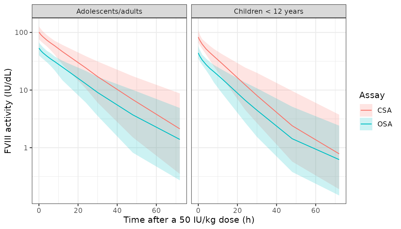
Median and 90% interval of FVIII activity by assay after a single 50 IU/kg dose. The one-stage assay reads about half the chromogenic activity of the drug, as in Figure S2 of the paper.
PKNCA computes Cmax, AUC0-72 and the 72 h concentration for each arm and assay. The paper reports no NCA, so the check is against the typical-value prediction: the median Cmax should sit near the typical-person value , where is 1 for CSA and 0.526 for OSA, at the arm’s median weight.
conc_df <- sim_pk |>
  dplyr::filter(!is.na(Cc)) |>
  select(id, arm, assay, time, Cc)
dose_df <- ev_coh |>
  dplyr::filter(evid == 1) |>
  select(id, arm, time, amt) |>
  tidyr::crossing(assay = c("CSA", "OSA"))

o_conc <- PKNCA::PKNCAconc(conc_df, Cc ~ time | arm + assay + id)
o_dose <- PKNCA::PKNCAdose(dose_df, amt ~ time | arm + assay + id)
intervals <- data.frame(start = 0, end = 72, cmax = TRUE, auclast = TRUE, clast.obs = TRUE)
nca <- PKNCA::pk.nca(PKNCA::PKNCAdata(o_conc, o_dose, intervals = intervals))

nca_sum <- as.data.frame(nca$result) |>
  group_by(arm, assay, PPTESTCD) |>
  summarise(median = median(PPORRES), .groups = "drop") |>
  tidyr::pivot_wider(names_from = PPTESTCD, values_from = median)

ini_pk <- setNames(mod_pk$iniDf$est, mod_pk$iniDf$name)
cmax_typ <- function(wt, assay) {
  vc <- exp(ini_pk[["lvc"]]) * (wt / 68)^ini_pk[["e_wt_vc"]]
  r <- ifelse(assay == "OSA", ini_pk[["e_assay_osa_cc"]], 1)
  50 * wt / vc * r + exp(ini_pk[["lrbase"]])
}
nca_sum <- nca_sum |>
  left_join(select(arms, arm, wt_med), by = "arm") |>
  mutate(cmax_typ = cmax_typ(wt_med, assay))

nca_sum |>
  transmute(
    arm, assay,
    cmax = signif(cmax, 3), cmax_typ = signif(cmax_typ, 3),
    auclast = signif(auclast, 3), clast.obs = signif(clast.obs, 3)
  ) |>
  dplyr::rename(
    "Arm" = arm,
    "Assay" = assay,
    "Cmax, PKNCA median (IU/dL)" = cmax,
    "Cmax, typical person (IU/dL)" = cmax_typ,
    "AUC0-72, PKNCA median (IU*h/dL)" = auclast,
    "C72h, PKNCA median (IU/dL)" = clast.obs
  ) |>
knitr::kable(caption = "PKNCA medians after a single 50 IU/kg dose.")| Arm | Assay | Cmax, PKNCA median (IU/dL) | Cmax, typical person (IU/dL) | AUC0-72, PKNCA median (IU*h/dL) | C72h, PKNCA median (IU/dL) |
|---|---|---|---|---|---|
| Adolescents/adults | CSA | 101.0 | 99.5 | 1670 | 2.120 |
| Adolescents/adults | OSA | 53.4 | 52.5 | 885 | 1.390 |
| Children < 12 years | CSA | 83.1 | 84.1 | 1010 | 0.782 |
| Children < 12 years | OSA | 44.1 | 44.4 | 554 | 0.621 |
Residual FVIII from a pre-study dose
For persons whose FVIII before the first study dose exceeded 1 IU/dL,
the model adds residual FVIII from an unknown earlier dose, 1.41 IU/dL
at the first record (typical value; IIV variance 3.505), decaying at the
person’s terminal disposition rate. In the packaged model this is a unit
dose into the prior_dose state at the first record, scaled
by its bioavailability. Persons without such a pre-dose level receive no
prior_dose record.
ev_prior <- bind_rows(
  rxode2::et(amt = 1, cmt = "prior_dose") |> as.data.frame(),
  rxode2::et(amt = 3500, time = 0, cmt = "central") |> as.data.frame(),
  rxode2::et(seq(0, 96, by = 1), cmt = "central") |> as.data.frame()
) |>
  arrange(time, desc(evid)) |>
  mutate(id = 1L, WT = 70, VWF = 113, ASSAY_OSA = 0)
ev_none <- ev_prior |>
  dplyr::filter(is.na(cmt) | cmt != "prior_dose") |>
  mutate(id = 2L)

prior_sim <- rxode2::rxSolve(
  rxode2::zeroRe(mod_pk), bind_rows(ev_prior, ev_none),
  returnType = "data.frame"
) |>
  suppressWarnings() |>
  suppressMessages() |>
  mutate(person = ifelse(id == 1, "Pre-dose FVIII > 1 IU/dL", "No residual pre-study FVIII"))

beta_typ <- prior_sim$beta_term[1]
stopifnot(
  # The residual term starts at EXTR and decays exactly as exp(-beta * t).
  abs(prior_sim$prior_dose[prior_sim$id == 1 & prior_sim$time == 48] -
    exp(ini_pk[["lfprior_dose"]]) * exp(-beta_typ * 48)) < 1e-6,
  all(prior_sim$prior_dose[prior_sim$id == 2] == 0)
)

ggplot(prior_sim, aes(time, Cc, colour = person)) +
  geom_line() +
  scale_y_log10() +
  labs(x = "Time (h)", y = "CSA FVIII activity (IU/dL)", colour = NULL) +
  theme_bw() +
  theme(legend.position = "bottom")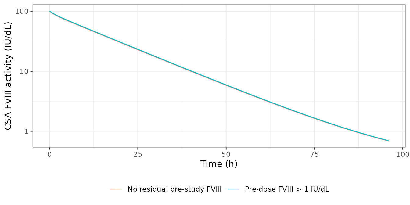
Bleeding RTTE validation
Hazard at constant FVIII (Figure 1)
Figure 1 shows the typical hazard for a constant FVIII level: 3.0 bleeds per year after one year at 1 IU/dL (panel a), and 3.3, 3.0, 1.65 and about 1.0 bleeds per year after one year at 0, 1, 8.9 (the IC50) and 20 IU/dL (panel b and Results). A constant FVIII level is obtained from the packaged model by giving no dose and setting the endogenous level to the target.
const_levels <- c(0, 1, 8.90353, 20)
grid_t <- c(seq(0, 24 * 10, by = 2), seq(24 * 11, 24 * 375, by = 24))
const_sim <- bind_rows(lapply(seq_along(const_levels), function(i) {
  ev <- rxode2::et(grid_t, cmt = "central") |>
    as.data.frame() |>
    mutate(id = i, WT = 70, VWF = 113)
  rxode2::rxSolve(
    rxode2::zeroRe(mod_bl), ev,
    params = c(lrbase = log(max(const_levels[i], 1e-12))),
    returnType = "data.frame"
  ) |>
    suppressWarnings() |>
    suppressMessages() |>
    mutate(fviii = const_levels[i])
}))

fig1 <- const_sim |>
  dplyr::filter(time == 24 * 365) |>
  transmute(fviii, haz_sim = hazard * 24 * 365) |>
  mutate(haz_pub = c(3.3, 3.0, 3.3 / 2, 1.0))

fig1 |>
  mutate(fviii = signif(fviii, 3), haz_sim = signif(haz_sim, 3)) |>
  dplyr::rename(
    "Constant FVIII (IU/dL)" = fviii,
    "Hazard at 1 year, model (per year)" = haz_sim,
    "Figure 1 / Results (per year)" = haz_pub
  ) |>
knitr::kable(caption = "Typical bleeding hazard after one year at a constant FVIII level.")| Constant FVIII (IU/dL) | Hazard at 1 year, model (per year) | Figure 1 / Results (per year) |
|---|---|---|
| 0.0 | 3.27 | 3.30 |
| 1.0 | 2.94 | 3.00 |
| 8.9 | 1.64 | 1.65 |
| 20.0 | 1.01 | 1.00 |
stopifnot(
  # Deterministic: lambda, gamma and IC50 all enter. The published values
  # are rounded to two significant figures.
  all(abs(fig1$haz_sim / fig1$haz_pub - 1) < 0.04)
)
const_sim |>
  dplyr::filter(fviii == 1, time > 0) |>
  ggplot(aes(time / 24, hazard * 24 * 365)) +
  geom_line(colour = "steelblue") +
  coord_cartesian(ylim = c(0, 23)) +
  labs(x = "Time (days)", y = "Bleeding hazard (per year)") +
  theme_bw()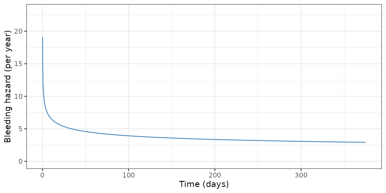
Replicates Figure 1a of Bukkems 2023: typical bleeding hazard at a constant FVIII level of 1 IU/dL (point estimate only; the paper’s band is the parameter uncertainty).
lam_y <- exp(mod_bl$iniDf$est[mod_bl$iniDf$name == "llam_haz"]) * 24 * 365
gam <- exp(mod_bl$iniDf$est[mod_bl$iniDf$name == "lgam_haz"])
ic50 <- exp(mod_bl$iniDf$est[mod_bl$iniDf$name == "lic50"])
data.frame(fviii = seq(0, 50, by = 0.5)) |>
  mutate(hazard = lam_y * gam * lam_y^(gam - 1) * (1 - fviii / (fviii + ic50))) |>
  ggplot(aes(fviii, hazard)) +
  geom_line(colour = "steelblue") +
  geom_point(data = fig1, aes(fviii, haz_sim)) +
  labs(x = "Constant FVIII level (IU/dL)", y = "Bleeding hazard after 1 year (per year)") +
  theme_bw()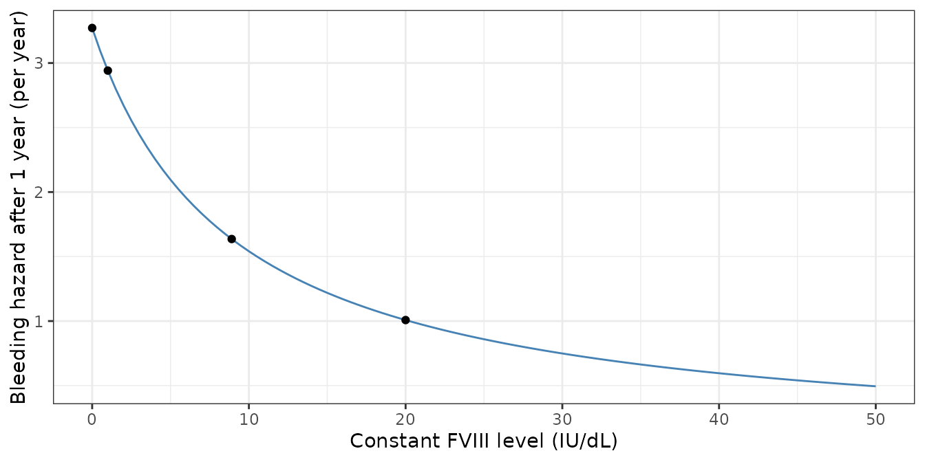
Replicates Figure 1b of Bukkems 2023 (the closed-form curve; the points are the packaged model’s solves from the previous chunk).
Annual bleeding rate at maintained trough levels (Figure 4)
Figure 4 simulates 1000 persons of 70 kg with typical PK parameters dosed every 72 h to maintain troughs of 1, 3, 5, 10 and 20 IU/dL, and reports the annual bleeding rate and the percentage with zero bleeds (20%, 31%, 37%, 48% and 59%, printed above the boxes). The Results and Discussion add the median ABR with its 90% prediction interval: 2 (0-17), 1 (0-11) and 1 (0-8) at troughs of 1, 3 and 5 IU/dL.
Successive bleeds are independent, so the number of bleeds in the first year is Poisson with mean equal to the cumulative hazard . With typical PK, , where is the typical cumulative hazard, because the random effect sits on and enters the hazard as . The ABR distribution is then a Poisson mixture over , computed here exactly by integration on a fine grid – no random draws are needed.
ev_f4 <- bind_rows(lapply(seq_len(nrow(trough_tab)), function(i) {
  rxode2::et(amt = trough_tab$dose[i], ii = 72, addl = 122, cmt = "central") |>
    rxode2::et(c(0, 24 * 365), cmt = "central") |>
    as.data.frame() |>
    mutate(id = i, WT = 70, VWF = 113)
}))
H0 <- rxode2::rxSolve(rxode2::zeroRe(mod_bl), ev_f4, returnType = "data.frame") |>
  suppressWarnings() |>
  suppressMessages() |>
  dplyr::filter(time == 24 * 365) |>
  arrange(id) |>
  pull(cumhaz)

omega_haz <- mod_bl$omega["etallam_haz", "etallam_haz"]
z <- seq(-8, 8, by = 0.005)
wz <- dnorm(z) * 0.005
abr_mixture <- function(H, mult) {
  k <- 0:400
  pk <- vapply(k, function(kk) sum(dpois(kk, H * mult) * wz), numeric(1))
  cdf <- cumsum(pk)
  c(
    p0 = 100 * pk[1],
    median = k[which(cdf >= 0.5)[1]],
    p05 = k[which(cdf >= 0.05)[1]],
    p95 = k[which(cdf >= 0.95)[1]]
  )
}
# Random effect on lambda inside the Weibull (the control stream).
f4 <- t(vapply(H0, abr_mixture, numeric(4), mult = exp(gam * sqrt(omega_haz) * z)))
# Random effect multiplying the whole hazard (Equation 1 as printed).
f4_eq1 <- t(vapply(H0, abr_mixture, numeric(4), mult = exp(sqrt(omega_haz) * z)))

fig4 <- data.frame(
  trough = trough_tab$trough_pub,
  H0 = H0,
  p0 = f4[, "p0"], p0_eq1 = f4_eq1[, "p0"],
  p0_pub = c(20, 31, 37, 48, 59),
  median = f4[, "median"],
  pi90 = paste0(f4[, "p05"], "-", f4[, "p95"]),
  pub = c("2 (0-17)", "1 (0-11)", "1 (0-8)", "1", "not stated")
)

fig4 |>
  mutate(across(c(H0, p0, p0_eq1), \(x) signif(x, 3))) |>
  dplyr::rename(
    "Trough (IU/dL)" = trough,
    "Typical 1-year cumulative hazard" = H0,
    "Zero bleeds, model (%)" = p0,
    "Zero bleeds, eta on whole hazard (%)" = p0_eq1,
    "Zero bleeds, Figure 4 (%)" = p0_pub,
    "Median ABR, model" = median,
    "90% PI, model" = pi90,
    "Median ABR (90% PI), paper" = pub
  ) |>
knitr::kable(caption = "First-year bleeds at maintained trough levels, 70 kg, typical PK.")| Trough (IU/dL) | Typical 1-year cumulative hazard | Zero bleeds, model (%) | Zero bleeds, eta on whole hazard (%) | Zero bleeds, Figure 4 (%) | Median ABR, model | 90% PI, model | Median ABR (90% PI), paper |
|---|---|---|---|---|---|---|---|
| 1 | 2.450 | 20.1 | 23.5 | 20 | 2 | 0-19 | 2 (0-17) |
| 3 | 1.460 | 30.3 | 32.6 | 31 | 1 | 0-12 | 1 (0-11) |
| 5 | 1.080 | 37.0 | 38.4 | 37 | 1 | 0-9 | 1 (0-8) |
| 10 | 0.677 | 48.1 | 47.9 | 48 | 1 | 0-6 | 1 |
| 20 | 0.393 | 60.6 | 58.7 | 59 | 0 | 0-4 | not stated |
stopifnot(
  # Exact integration, no random draws: the percentages with zero bleeds
  # match the Figure 4 annotations (which carry the paper's own 1000-person
  # sampling noise, about +/- 1.5 points).
  all(abs(fig4$p0 - fig4$p0_pub) < 2.5),
  all(fig4$median[1:4] == c(2, 1, 1, 1))
)
The first-year zero-bleed percentages and median ABRs reproduce Figure 4 and the Results. The model’s 90% prediction intervals are slightly wider at their upper end (19, 12 and 9 bleeds against 17, 11 and 8); the 95th percentile of 1000 simulated persons from this heavy-tailed mixture varies by a few bleeds between simulations. Placing the random effect on the whole hazard, as Equation 1 is printed, moves the zero-bleed percentages by up to 3.4 points and fits the low-trough values less well (23.5% against the published 20% at 1 IU/dL); the packaged model follows the control stream (see Assumptions).
abr_dist <- bind_rows(lapply(seq_along(H0), function(i) {
  k <- 0:30
  data.frame(
    trough = factor(trough_tab$trough_pub[i]),
    abr = k,
    prob = vapply(k, function(kk) {
      sum(dpois(kk, H0[i] * exp(gam * sqrt(omega_haz) * z)) * wz)
    }, numeric(1))
  )
}))
ggplot(abr_dist, aes(abr, prob)) +
  geom_col(fill = "steelblue") +
  facet_wrap(~trough, nrow = 1, labeller = label_both) +
  coord_cartesian(xlim = c(0, 15)) +
  labs(x = "Bleeds in the first year", y = "Probability") +
  theme_bw()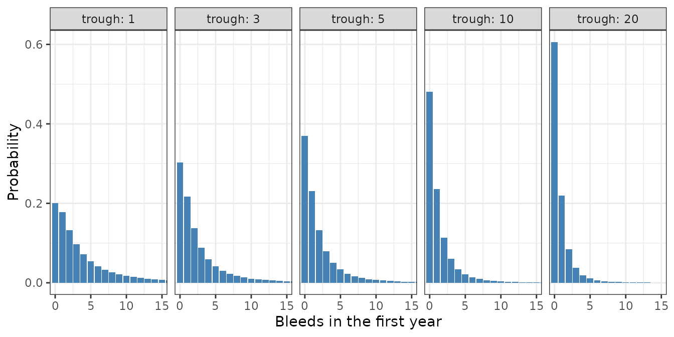
Distribution of the first-year bleed count underlying Figure 4 of Bukkems 2023 (shown as probabilities rather than boxplots).
FVIII and hazard for the two illustrative persons (Figure 2)
Figure 2 shows two persons from the dataset: A (38 kg, 13 years, 1000 IU twice weekly) and B (60 kg, 19 years, 2000 IU twice weekly). Their individual parameters are not published; the typical-value profiles below use their weight and a VWF predicted from their age with the paper’s regression (Appendix S2: 79.367 + 1.6672 x age).
persons <- data.frame(
  person = c("A: 38 kg, 1000 IU twice weekly", "B: 60 kg, 2000 IU twice weekly"),
  wt = c(38, 60), age = c(13, 19), dose = c(1000, 2000)
)
fig2 <- bind_rows(lapply(seq_len(nrow(persons)), function(i) {
  ev <- rxode2::et(amt = persons$dose[i], ii = 84, addl = 120, cmt = "central") |>
    rxode2::et(seq(24 * 330, 24 * 358, by = 1), cmt = "central") |>
    as.data.frame() |>
    mutate(id = i, WT = persons$wt[i], VWF = 79.367 + 1.6672 * persons$age[i])
  rxode2::rxSolve(rxode2::zeroRe(mod_bl), ev, returnType = "data.frame") |>
    suppressWarnings() |>
    suppressMessages() |>
    mutate(person = persons$person[i])
}))

fig2 |>
  transmute(
    person, day = time / 24,
    `FVIII activity (IU/dL)` = Cc,
    `Bleeding hazard (per year)` = hazard * 24 * 365
  ) |>
  tidyr::pivot_longer(-c(person, day)) |>
  ggplot(aes(day, value)) +
  geom_line(colour = "steelblue") +
  facet_grid(name ~ person, scales = "free_y") +
  labs(x = "Time since study start (days)", y = NULL) +
  theme_bw()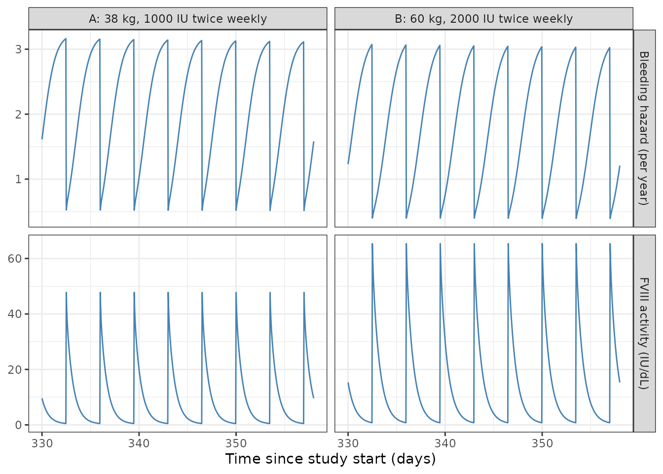
Typical-value analogue of the top and middle panels of Figure 2 of Bukkems 2023: the hazard rises as FVIII activity falls between doses.
Assumptions and deviations
- Parameter values. The unrounded final estimates of the two NONMEM control streams (Appendices S2 and S3) are used; they round to every Table 2 and Table 3 value, with one exception: the IIV of the residual previous-dose level, 3.505 in the control stream, converts to 568 CV%, whereas Table 2 prints 596.6 CV%. The control-stream variance is used.
- Where the hazard random effect enters. Equation 1 multiplies the whole hazard by , but the control stream places the random effect on the Weibull scale, , so it enters the hazard as . The control stream is the model that produced the estimates (the omega of 2.478 belongs to this placement), and it reproduces the Figure 4 zero-bleed percentages slightly better than the printed one.
- Residual error model. The control stream’s error components are independent normal terms, so their variances add; the packaged model computes the total SD per row and scales it by the individual residual-error random effect. Two features cannot be carried: (1) the CSA and OSA proportional terms are correlated (covariance 0.0298, a correlation of about 1) within a sample measured by both assays, which matters only when simulating paired assays of the same sample; and (2) the separate error terms for repeated measurements of the same sample have equal variances, so they reduce to one term per assay. Table 2 prints the two “multiple measurements” rows with OSA and CSA interchanged relative to the control stream (13.3% belongs to the CSA terms EPS(5)/EPS(6), 21.4% to the OSA terms EPS(7)-EPS(9)); the control stream is followed. Table 2’s ‘Additive error CSA’ of 0.55 IU/dL is the variance (0.546); the SD is 0.739 IU/dL. The OSA additive term was held at zero and is omitted.
- Weight centring. The Table 2 footnote says typical values refer to a 70 kg person, but its equations and the control stream centre on 68 kg; 68 kg is used.
- VWF imputation. For the 154 persons without a VWF measurement, the source imputed VWF inside the model from age (79.367 + 1.6672 x age, with a random effect of variance 1931 held constant). This missing-data device is not part of the packaged models; supply VWF for every simulated person. Figure S1 prints the regression as 79.58 + 1.66 x age; the control-stream coefficients are used where needed here.
-
Residual pre-study FVIII. The source switches the
decaying residual term on with a data flag for persons whose FVIII
before the first study dose exceeded 1 IU/dL. The packaged model encodes
it as a unit dose into the
prior_dosestate at the first record, which reproduces exactly; give that record only to such persons. The RTTE model does not include this term. -
RTTE output and likelihood. The source fits the
RTTE likelihood with right censoring at the end of follow-up and
interval censoring over the day for bleeds with an unknown time. The
packaged RTTE file exposes the hazard, the cumulative hazard and the
survivor function
surfor simulation, and attaches a placeholder additive error (SD 0.001) tosurthat is not from the source.suris the probability of no bleed since time zero; the source’s survival since the last bleed isexp(-(cumhaz - cumhaz at the last bleed)). - Hazard time origin. The Weibull time is time since the person’s first record (study start) and is not reset after a bleed. The source’s offset of inside is kept.
-
Sequential estimation. In the source the RTTE model
was driven by each person’s empirical Bayes PK estimates. The packaged
RTTE file embeds the PK model with its IIV, so a simulation draws new PK
parameters for each virtual person; fix them with
params =to reproduce a known person. -
Covariates on the hazard. Body weight, VWF, region,
hemophilic arthropathy and the pre-study annual bleeding rate were
screened in a full fixed-effects covariate model; only the pre-study
rate had a clinically important effect, and none is in the final RTTE
model (Table 3; Appendix S3). Their effect sizes are reported only
graphically (Figure 3), so they are documented in
covariatesDataExcludedrather than encoded. - Virtual cohorts. Weight and VWF are drawn log-normally around the trial medians of Table 1; the PKNCA cohort is not meant to reproduce a published table, since the paper reports no NCA.