Linerixibat C4 and GSRS diarrhea bother (Carreno 2025)
Source:vignettes/articles/Carreno_2025_linerixibat.Rmd
Carreno_2025_linerixibat.RmdModel and source
- Citation: Carreno F, Mehta R, Sherman AR, Collins J, Swift B. Analysis of C4 Concentrations to Predict Impact of Patient-Reported Diarrhea Associated With the Ileal Bile Acid Transporter Inhibitor Linerixibat. CPT Pharmacometrics Syst Pharmacol. 2025;14(3):596-605. doi:10.1002/psp4.13300
- Description: Kinetic-pharmacodynamic (K-PD) model of serum 7-alpha-hydroxy-4-cholesten-3-one (C4), a marker of bile acid synthesis, after oral linerixibat (an ileal bile acid transporter inhibitor) in healthy volunteers and patients with primary biliary cholangitis, linked to a longitudinal proportional-odds model of the patient-reported GSRS diarrhea-bother score (Question 11, scores 1-7) in patients with primary biliary cholangitis and pruritus (Carreno 2025). Linerixibat is minimally absorbed, so the dose enters a virtual compartment that empties first-order at a fixed rate; the dose rate leaving it stimulates the zero-order C4 synthesis rate through an Emax function. C4 synthesis follows a dual-cosine diurnal rhythm (8-h and 12-h periods) whose first amplitude falls with the individual baseline C4. The cumulative logits of the GSRS score carry an Emax function of the model-predicted C4 concentration and one between-subject random effect shared by all thresholds.
- Article: https://doi.org/10.1002/psp4.13300 (open access, PMC11919258)
Linerixibat is an ileal bile acid transporter (IBAT) inhibitor with an oral bioavailability of about 0.05%, so no plasma PK model drives the response. The dose enters a virtual compartment (a kinetic-pharmacodynamic, K-PD, model) whose output rate stimulates the synthesis of serum 7-alpha-hydroxy-4-cholesten-3-one (C4), the bile acid synthesis marker. The predicted C4 then drives a proportional-odds model of the patient-reported GSRS Question 11 score, “Have you been bothered by diarrhea during the past week?”, scored 1 (no discomfort) to 7 (very severe discomfort).
Population
The C4 K-PD model was fitted to 3292 C4 concentrations from 255 participants in five studies (Table 1 and Table S1): 86 healthy volunteers in three phase 1 studies (NCT01416324 single doses 0.1-60 mg and 30 mg BID; NCT01607385 3-90 mg BID for 12 days; NCT02801981 single 10-180 mg doses in Japanese volunteers) and 169 patients with primary biliary cholangitis (PBC) and pruritus (NCT01899703, 45 then 90 mg BID; GLIMMER, NCT02966834, 20, 90 or 180 mg QD or 40 or 90 mg BID for 12 weeks after a 4-week placebo run-in). 63% of the participants were female; geometric mean age ranged from 31 to 55 years and geometric mean body weight from 62.8 to 82.2 kg across studies. Baseline C4 geometric means were 7.4-14.1 ng/mL. The GSRS proportional-odds model used the 147 GLIMMER patients (713 run-in and 1640 treatment-period observations).
The same information is available programmatically via
readModelDb("Carreno_2025_linerixibat")()$population.
Source trace
Every ini() value carries an in-file comment pointing to
its source. The structural equations are in Supplementary Methods S1
(Equation 1 and the virtual-compartment equations) and in Figure 1 of
the article.
| Equation / parameter | Value | Source location |
|---|---|---|
d/dt(depot_kpd) = -KDE * A;
DR = KDE * A
|
n/a | Supplementary Methods S1, virtual compartment |
EFF = Emax * DR / (EDK50 + DR) |
n/a | Supplementary Methods S1; Figure 1 |
d/dt(C4) = Kin * (1 + CYR1 + CYR2) * (1 + EFF) - Kout * C4 |
n/a | Supplementary Equation 1; Figure 1 |
CYR1 = AMP * cos((t - Tpeak1) * 2 * pi / 8),
CYR2 = AMP2 * cos((t - Tpeak2) * 2 * pi / 12)
|
n/a | Supplementary Methods S1, diurnal variation definition |
logit P(Y <= s) = f_s + eta |
n/a | Supplementary Methods S1, proportional-odds model |
lkel (KDE) |
0.110 1/h, fixed | Table 2 |
lemax (Emax) |
5.55 | Table 2 |
ledk50 (EDK50) |
3.03 mg/h | Table 2 |
lrbase (Baseline) |
11.9 ng/mL | Table 2 |
lkout (Kout) |
0.135 1/h | Table 2 |
kin_circ_famp1 (Amplitude1) |
0.268 | Table 2 |
tacro1 (Acrophase1) |
5.77 h | Table 2 |
e_rbase_kin_circ_famp1 (effect of baseline C4 on
amplitude) |
-0.0130 | Table 2 (functional form not printed; see Assumptions) |
kin_circ_famp2 (Amplitude2) |
0.0227 | Table 2 |
tacro2 (Acrophase2) |
21.7 h | Table 2 |
logite0 |
4.05 (= -(-4.05)) | Table 2, intercept m = 2 |
logitstep1 to logitstep5
|
1.26, 0.983, 1.15, 1.11, 1.53 | Table 2, intercepts m = 3 to 7 |
lemax_gsrs_diarrhea |
11.6 | Table 2, PO Emax |
lec50_gsrs_diarrhea |
42.9 ng/mL | Table 2, PO EC50 |
etalrbase |
log(1 + 0.892^2) = 0.586 (89.2% CV) | Table 2 |
etalemax |
log(1 + 0.558^2) = 0.269 (55.8% CV) | Table 2 |
etaledk50 |
log(1 + 3.58^2) = 2.63 (358% CV) | Table 2 |
etalogite0 |
5.44^2 = 29.6 (SD 5.44) | Table 2, IIV on the m = 2 intercept |
addSd_c4 |
0.000492 ng/mL, fixed | Table 2 |
propSd_c4 |
0.448 | Table 2 |
Typical-value checks
mod <- readModelDb("Carreno_2025_linerixibat")
mod_typ <- rxode2::zeroRe(mod)
#> ℹ parameter labels from comments will be replaced by 'label()'
ini_val <- rxode2::rxode(mod)$theta
#> ℹ parameter labels from comments will be replaced by 'label()'
Placebo: the diurnal rhythm averages to the baseline
Without drug the model is linear, so once the start-up transient has
decayed the 24-hour mean of C4 equals Kin / Kout, the
baseline of 11.9 ng/mL. Both sides use the same parameters, so the check
is tight.
ev_pbo <- rxode2::et(amt = 0, cmt = "depot_kpd") |>
  rxode2::et(seq(0, 10 * 24, by = 0.1), cmt = "c4")
s_pbo <- rxode2::rxSolve(mod_typ, ev_pbo, returnType = "data.frame")
#> ℹ omega/sigma items treated as zero: 'etalrbase', 'etalemax', 'etaledk50', 'etalogite0'
day10 <- s_pbo |> filter(time >= 9 * 24, time < 10 * 24)
mean_day10 <- mean(day10$c4)
stopifnot(abs(mean_day10 / exp(ini_val[["lrbase"]]) - 1) < 1e-3)
c(mean = mean_day10, min = min(day10$c4), max = max(day10$c4))
#>     mean      min      max
#> 11.90000 11.30740 12.50384

ggplot(day10, aes(time - 9 * 24, c4)) +
  geom_line() +
  labs(
    x = "Time within day 10 (h after the time-0 reference)",
    y = "Typical C4 (ng/mL)",
    title = "Typical diurnal C4 profile without drug"
  )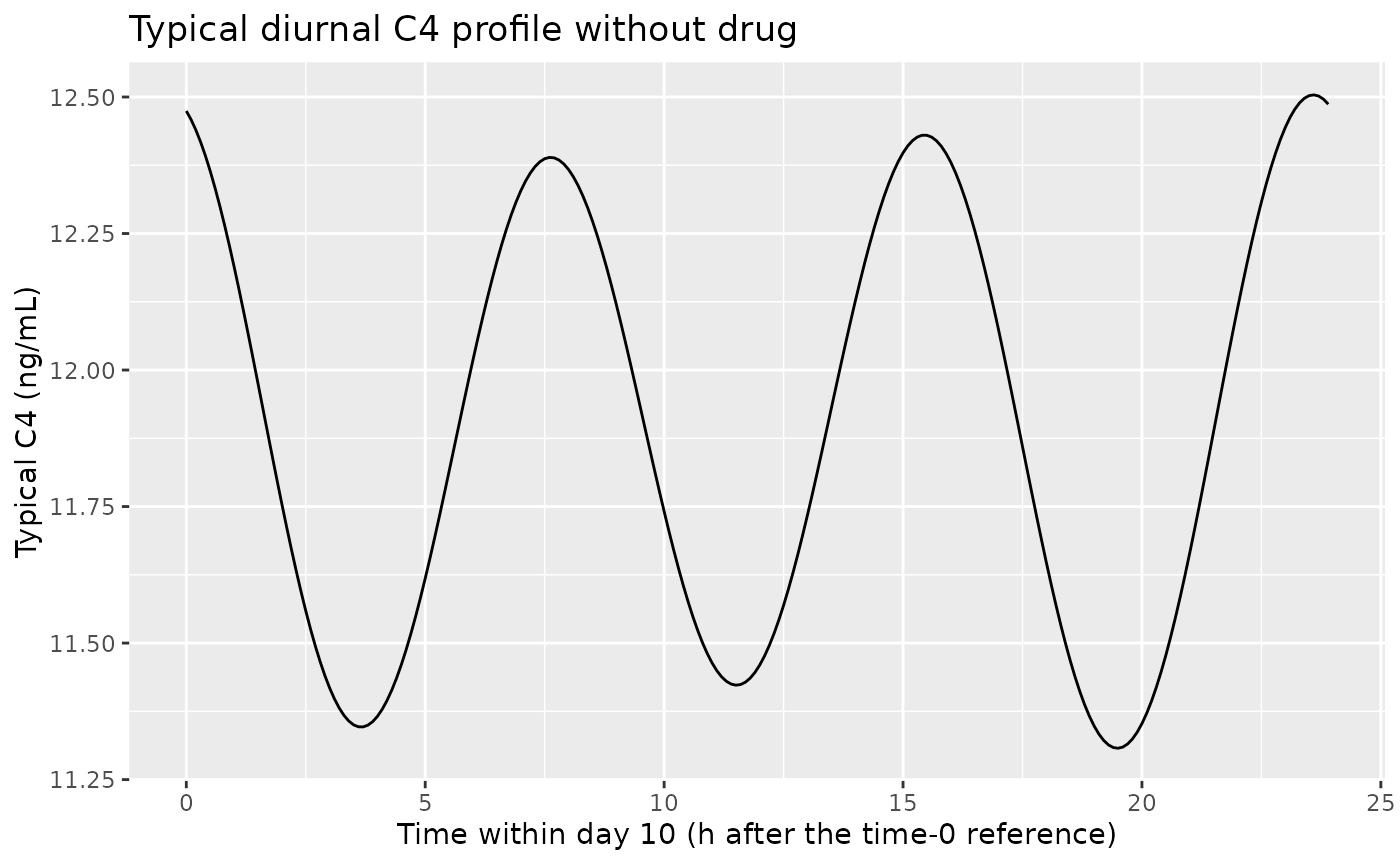
The attenuation of the 8-h rhythm by C4 turnover (Kout = 0.135 1/h) keeps the within-day swing to a few percent.
Constant dose rate: closed-form steady state
A zero-order infusion into the virtual compartment at R
mg/h holds the dose rate at R, so the 24-hour mean of C4
settles at Baseline * (1 + Emax * R / (EDK50 + R)).
rate <- 5 # mg/h
ev_inf <- rxode2::et(amt = rate * 24 * 20, rate = rate, cmt = "depot_kpd") |>
  rxode2::et(seq(0, 20 * 24, by = 0.1), cmt = "c4")
s_inf <- rxode2::rxSolve(mod_typ, ev_inf, returnType = "data.frame")
#> ℹ omega/sigma items treated as zero: 'etalrbase', 'etalemax', 'etaledk50', 'etalogite0'
mean_inf <- s_inf |> filter(time >= 18 * 24, time < 19 * 24) |> pull(c4) |> mean()
expected <- exp(ini_val[["lrbase"]]) *
  (1 + exp(ini_val[["lemax"]]) * rate / (exp(ini_val[["ledk50"]]) + rate))
stopifnot(abs(mean_inf / expected - 1) < 1e-3)
c(simulated = mean_inf, closed_form = expected)
#>   simulated closed_form
#>    53.02391    53.02391
Twice-daily versus once-daily dosing
The article reports that the twice-daily regimens raised C4 by approximately 24% compared with a similar once-daily total daily dose (90 mg BID versus 180 mg QD). The typical-subject morning trough after four weeks reproduces it.
arms <- tibble::tribble(
  ~arm,         ~amt, ~ii,
  "Placebo",       0,  24,
  "20 mg QD",     20,  24,
  "90 mg QD",     90,  24,
  "180 mg QD",   180,  24,
  "40 mg BID",    40,  12,
  "90 mg BID",    90,  12
) |>
  mutate(arm = factor(arm, levels = arm))

typ_trough <- function(amt, ii) {
  ev <- rxode2::et(amt = amt, ii = ii, addl = 28 * 24 / ii - 1, cmt = "depot_kpd") |>
    rxode2::et(27 * 24, cmt = "c4")
  s <- rxode2::rxSolve(mod_typ, ev, returnType = "data.frame")
  s$c4[s$time == 27 * 24]
}
arms$typical_trough <- mapply(typ_trough, arms$amt, arms$ii)
#> ℹ omega/sigma items treated as zero: 'etalrbase', 'etalemax', 'etaledk50', 'etalogite0'
#> ℹ omega/sigma items treated as zero: 'etalrbase', 'etalemax', 'etaledk50', 'etalogite0'
#> ℹ omega/sigma items treated as zero: 'etalrbase', 'etalemax', 'etaledk50', 'etalogite0'
#> ℹ omega/sigma items treated as zero: 'etalrbase', 'etalemax', 'etaledk50', 'etalogite0'
#> ℹ omega/sigma items treated as zero: 'etalrbase', 'etalemax', 'etaledk50', 'etalogite0'
#> ℹ omega/sigma items treated as zero: 'etalrbase', 'etalemax', 'etaledk50', 'etalogite0'
knitr::kable(
  arms |>
    select(arm, typical_trough) |>
    dplyr::rename("Regimen" = arm, "Typical morning trough C4, day 28 (ng/mL)" = typical_trough),
  digits = 1
)| Regimen | Typical morning trough C4, day 28 (ng/mL) |
|---|---|
| Placebo | 12.5 |
| 20 mg QD | 20.3 |
| 90 mg QD | 35.9 |
| 180 mg QD | 46.6 |
| 40 mg BID | 44.4 |
| 90 mg BID | 57.6 |
Virtual GLIMMER cohort
The GLIMMER design is simulated: a 4-week placebo run-in followed by 12 weeks of linerixibat or placebo dosed in the morning (the second BID dose 12 h later), with fasting morning C4 samples taken before the dose. Each arm has 200 virtual patients drawn from the population model.
n_per_arm <- 200
run_in <- 28 * 24
obs_times <- c(0, 4, 5, 8, 12, 16) * 7 * 24

make_arm <- function(i, n) {
  a <- arms[i, ]
  ids <- (i - 1) * n + seq_len(n)
  obs <- tidyr::expand_grid(id = ids, time = obs_times) |>
    mutate(evid = 0, amt = 0, cmt = "c4", ii = 0, addl = 0)
  if (a$amt > 0) {
    dose <- tibble(
      id = ids, time = run_in, evid = 1, amt = a$amt, cmt = "depot_kpd",
      ii = a$ii, addl = 12 * 7 * 24 / a$ii - 1
    )
    obs <- bind_rows(obs, dose)
  }
  obs |> mutate(arm = a$arm)
}
events <- bind_rows(lapply(seq_len(nrow(arms)), make_arm, n = n_per_arm)) |>
  arrange(id, time, desc(evid)) |>
  mutate(arm = as.character(arm))
stopifnot(!anyDuplicated(events[, c("id", "time", "evid")]))Replicate published figures
Figure 3: C4 trough by regimen
fig3 <- sim |>
  group_by(arm, week = time / (7 * 24)) |>
  summarise(mean_c4 = mean(c4), median_c4 = median(c4), .groups = "drop") |>
  filter(week != 5)

ggplot(fig3, aes(week, mean_c4, colour = arm)) +
  geom_line(linetype = "dashed") +
  geom_point() +
  labs(
    x = "Study week", y = "Mean simulated C4 (ng/mL)", colour = "Linerixibat dose",
    title = "Mean morning trough C4 by GLIMMER regimen",
    caption = "Replicates Figure 3 of Carreno 2025."
  )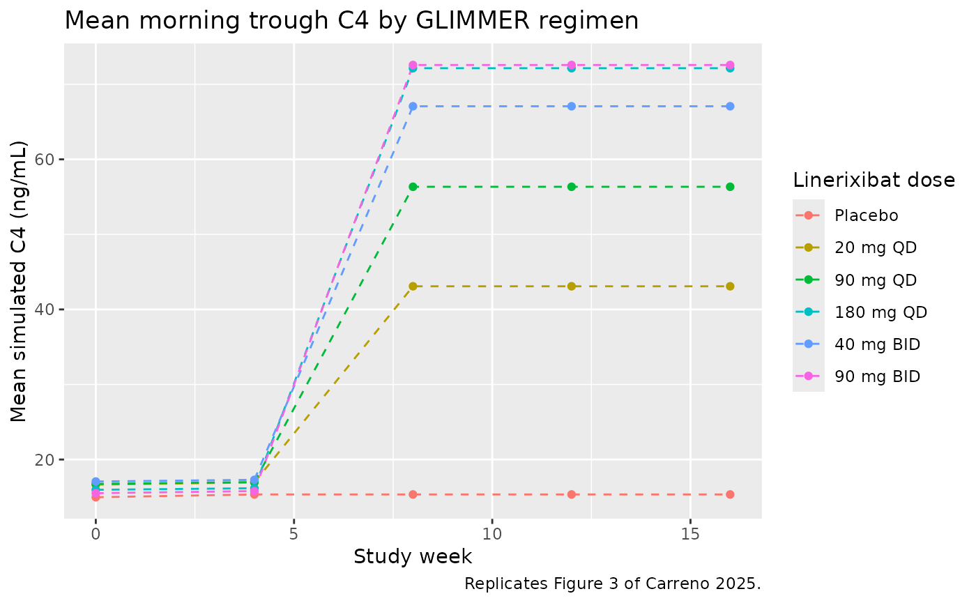
The article’s Figure 3 shows means of about 19 (placebo), 34 (20 mg QD), 45 (90 mg QD), 50 (40 mg BID), 51 (180 mg QD) and 56 ng/mL (90 mg BID), and the Results text gives medians (90% prediction intervals) of 16.7 (5.08, 41.1), 27.3 (8.21, 82.8), 36.2 (11.1, 110), 39.7 (12.4, 120), 40.9 (12.8, 121) and 44.2 (14.4, 131) ng/mL in the same order.
tab3 <- sim |>
  filter(time == 12 * 7 * 24) |>
  group_by(arm) |>
  summarise(
    mean = mean(c4),
    median = median(sim),
    p05 = quantile(sim, 0.05),
    p95 = quantile(sim, 0.95),
    .groups = "drop"
  ) |>
  mutate(
    paper_mean = c(19, 34, 45, 51, 50, 56),
    paper_median = c(16.7, 27.3, 36.2, 40.9, 39.7, 44.2),
    ratio_model = median / median[arm == "Placebo"],
    ratio_paper = paper_median / paper_median[arm == "Placebo"]
  )
knitr::kable(
  tab3 |>
    dplyr::rename(
      "Regimen" = arm, "Mean C4" = mean, "Median C4 (with residual)" = median,
      "5th pct" = p05, "95th pct" = p95, "Paper mean (Fig. 3)" = paper_mean,
      "Paper median (Results)" = paper_median,
      "Median / placebo, model" = ratio_model, "Median / placebo, paper" = ratio_paper
    ),
  digits = 2
)| Regimen | Mean C4 | Median C4 (with residual) | 5th pct | 95th pct | Paper mean (Fig. 3) | Paper median (Results) | Median / placebo, model | Median / placebo, paper |
|---|---|---|---|---|---|---|---|---|
| Placebo | 15.34 | 11.24 | 2.56 | 39.60 | 19 | 16.7 | 1.00 | 1.00 |
| 20 mg QD | 43.09 | 24.72 | 2.96 | 137.64 | 34 | 27.3 | 2.20 | 1.63 |
| 90 mg QD | 56.34 | 32.24 | 5.72 | 181.11 | 45 | 36.2 | 2.87 | 2.17 |
| 180 mg QD | 72.14 | 42.69 | 3.98 | 231.85 | 51 | 40.9 | 3.80 | 2.45 |
| 40 mg BID | 67.07 | 44.40 | 5.26 | 221.40 | 50 | 39.7 | 3.95 | 2.38 |
| 90 mg BID | 72.57 | 42.83 | 6.22 | 213.36 | 56 | 44.2 | 3.81 | 2.65 |
The dose ordering and the BID-over-QD advantage are reproduced. The model’s placebo level is lower and its prediction interval wider than the article’s, and its active-to-placebo ratios are larger at the higher doses. The article’s simulation used the GLIMMER participants (Methods: “The demographics of participants in GLIMMER were used for all simulations”), whose observed baseline C4 had a geometric mean of 14.1 ng/mL (Table 1), and its narrow prediction intervals indicate that it drew on the participants’ individual parameter estimates rather than on fresh draws from the population distribution used here. Those individual estimates are not published, so the comparison above is made on the population model.
Probability of moderate-to-very-severe diarrhea bother
The article reports that, after the first week of dosing, the probability of a GSRS score of 4 or more rose over placebo by 9, 17, 20, 19 and 23 percentage points for 20, 90 and 180 mg QD and 40 and 90 mg BID. The marginal probability over the large between-subject random effect on the logits (SD 5.44) is integrated numerically for each simulated patient’s C4.
eta_sd <- sqrt(rxode2::rxode(mod)$omega["etalogite0", "etalogite0"])
#> ℹ parameter labels from comments will be replaced by 'label()'
eta_grid <- seq(-6, 6, length.out = 241) * eta_sd
w <- dnorm(eta_grid, sd = eta_sd)
w <- w / sum(w)
lp3 <- ini_val[["logite0"]] + ini_val[["logitstep1"]] + ini_val[["logitstep2"]]
marg_ge4 <- function(c4) {
  eff <- exp(ini_val[["lemax_gsrs_diarrhea"]]) * c4 /
    (exp(ini_val[["lec50_gsrs_diarrhea"]]) + c4)
  vapply(eff, function(e) sum(w * (1 - plogis(lp3 + eta_grid - e))), numeric(1))
}
pge4 <- sim |>
  filter(time == 5 * 7 * 24) |>
  mutate(p_ge4_marg = marg_ge4(c4)) |>
  group_by(arm) |>
  summarise(p_ge4 = mean(p_ge4_marg), .groups = "drop") |>
  mutate(
    increase_model = 100 * (p_ge4 - p_ge4[arm == "Placebo"]),
    increase_paper = c(NA, 9, 17, 20, 19, 23)
  )
knitr::kable(
  pge4 |>
    dplyr::rename(
      "Regimen" = arm, "P(score >= 4)" = p_ge4,
      "Increase over placebo, model (points)" = increase_model,
      "Increase over placebo, paper (points)" = increase_paper
    ),
  digits = 2
)| Regimen | P(score >= 4) | Increase over placebo, model (points) | Increase over placebo, paper (points) |
|---|---|---|---|
| Placebo | 0.28 | 0.00 | NA |
| 20 mg QD | 0.38 | 10.79 | 9 |
| 90 mg QD | 0.45 | 17.01 | 17 |
| 180 mg QD | 0.46 | 18.60 | 20 |
| 40 mg BID | 0.48 | 20.11 | 19 |
| 90 mg BID | 0.49 | 21.56 | 23 |
d_inc <- (pge4$increase_model - pge4$increase_paper)[-1]
stopifnot(
  abs(median(d_inc)) < 3,
  max(abs(d_inc)) < 6
)
These increments depend on the logit random effect being an SD of 5.44 (the Table 2 footnote reports the SD for additive random effects); reading 5.44 as a variance roughly doubles every increment.
Figure S4: typical probability of each score threshold versus C4
c4_grid <- seq(2, 100, by = 1)
eff_grid <- exp(ini_val[["lemax_gsrs_diarrhea"]]) * c4_grid /
  (exp(ini_val[["lec50_gsrs_diarrhea"]]) + c4_grid)
steps <- c(0, cumsum(unlist(ini_val[paste0("logitstep", 1:5)])))
s4 <- tidyr::expand_grid(k = 2:7, i = seq_along(c4_grid)) |>
  mutate(
    c4 = c4_grid[i],
    p = 1 - plogis(ini_val[["logite0"]] + steps[k - 1] - eff_grid[i]),
    threshold = factor(paste0("score >= ", k), levels = paste0("score >= ", 2:7))
  )
ggplot(s4, aes(c4, p, colour = threshold)) +
  geom_line() +
  labs(
    x = "Serum C4 (ng/mL)", y = "Typical probability", colour = NULL,
    title = "Typical-patient probability of reaching each GSRS score",
    caption = "Replicates Figure S4 of Carreno 2025 (the figure labels the thresholds one lower)."
  )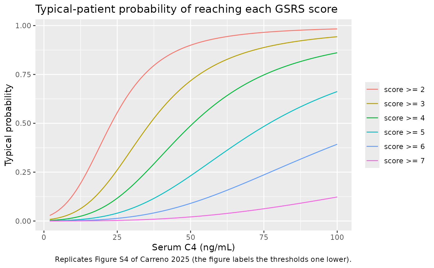
The curves match Figure S4 in the mid-range (for example the typical probability of a score of 2 or more is 0.38 at 19 ng/mL and 0.90 at 50 ng/mL, against about 0.37 and 0.89 read from the figure). Figure S4 sits somewhat higher than the Emax form at the lowest and highest C4 concentrations; the figure legend runs from “scores >= 1”, which the model can only match if each label denotes the next score up.
Assumptions and deviations
- Effect of baseline C4 on the 8-h amplitude. Table 2 reports an “effect of baseline C4 on amplitude” of -0.0130 but no equation. The maintainers chose to encode it as a linear change in the 8-h fractional amplitude per ng/mL of the individual baseline above the typical baseline of 11.9 ng/mL, so the typical amplitude is the tabulated 0.268. The uncentred linear form and a proportional centred form change the median morning trough C4 by less than 3% and the probability of a score of 4 or more by less than 0.5 points.
- Time axis of the cosines. Supplementary Equation 1 writes the rhythm in terms of “Time”. It is applied to the model time, with time 0 at the first dose on Day 1, as in the source datasets; acrophases are therefore hours after that reference rather than clock times.
- C4 initial condition. C4 starts at the individual baseline rather than on the periodic diurnal cycle; the transient is a few percent and decays within about a day.
-
Proportional-odds parameterisation. The article
reports intercepts for
P(score >= m), with m = 2 the intercept and m = 3..7 positive decrements. The model follows the library’slogit P(score <= m)convention, so the m = 2 intercept enters with its sign flipped aslogite0and the C4 Emax term is subtracted; the probabilities are identical. - C4 driving the GSRS model. The article links the models with the IPPSE method (individual K-PD parameters and their standard errors). Here the individual predicted C4 at the observation time drives the logits. The article’s simulations used fasting morning C4, so evaluate the GSRS probabilities at the pre-dose morning time.
- Logit random effect. Table 2 prints 5.44 for the intercept IIV; the table footnote states that additive random effects are reported as SDs, so the variance is 5.44^2 = 29.59. The reproduction of the article’s simulated increments above supports this reading.
- Population simulations. The article’s GLIMMER simulations used the GLIMMER participants; the cohort here is drawn from the population model, so absolute C4 levels differ (see Figure 3 above).