Efalizumab CD11a target engagement and PASI response (Chetty 2014)
Source:vignettes/articles/Chetty_2014_efalizumab_cd11a_pasi.Rmd
Chetty_2014_efalizumab_cd11a_pasi.RmdModels and source
ui_cd11a <- rxode2::rxode(readModelDb("Chetty_2014_efalizumab_cd11a_qsp"))
ui_pasi <- rxode2::rxode(readModelDb("Chetty_2014_efalizumab_pasi"))- Citation: Chetty M, Li L, Rose R, Machavaram K, Jamei M, Rostami-Hodjegan A, Gardner I. (2015). Prediction of the pharmacokinetics, pharmacodynamics, and efficacy of a monoclonal antibody, using a physiologically based pharmacokinetic FcRn model. Front Immunol 5:670. doi:10.3389/fimmu.2014.00670. PMCID PMC4283607. Every parameter value is from main-text Table 1. The Michaelis-Menten / quasi-steady-state target equations are the form Chetty 2014 attributes to its reference 23 (Gibiansky L, Gibiansky E, Kakkar T, Ma P. Approximations of the target-mediated drug disposition model and identifiability of model parameters. J Pharmacokinet Pharmacodyn 2008;35:573-591), and the paper enumerates their ingredients explicitly in the Methods bullet list (kon binding, koff dissociation, kint complex internalisation, saturation of binding sites, Ksyn synthesis and Kdeg degradation of CD11a, with Km subsuming kon, koff and kint). Chetty 2014 has no supplementary material and no erratum; the only linked item is a later ‘Comment in’ (AAPS J 2016;18:948-59). The companion efficacy model from the same paper is modellib(‘Chetty_2014_efalizumab_pasi’).
- Article: https://doi.org/10.3389/fimmu.2014.00670 (open access; PMCID PMC4283607)
Chetty 2014 built a three-layer model of efalizumab, a humanised anti-CD11a monoclonal antibody once licensed for moderate-to-severe plaque psoriasis:
- a whole-body Mechanistic FcRn PBPK disposition model in the Simcyp Simulator (Version 13 R1), which produces the efalizumab concentration-time profile;
- a CD11a target-turnover and target-engagement model, written in the Michaelis-Menten / quasi-steady-state approximation of target-mediated drug disposition of Gibiansky et al. 2008, which consumes that concentration and produces the free and total CD11a pools; and
- a PASI disease-progression model, a first-order asymptotic decay from the cohort baseline score to a treated steady-state asymptote.
Layers 2 and 3 are extracted here as two model files. Layer 1 is not extracted; the next section says why.
tibble::tibble(
  Model = c("Chetty_2014_efalizumab_cd11a_qsp", "Chetty_2014_efalizumab_pasi"),
  Layer = c("CD11a target turnover + MM/QSS engagement", "PASI first-order asymptotic progression"),
  State = c("total_target (umol/L)", "pasi (0-72 score)"),
  `Paper figure` = c("Figure 3", "Figure 4")
) |>
knitr::kable(caption = "The two model files this paper contributed.")| Model | Layer | State | Paper figure |
|---|---|---|---|
| Chetty_2014_efalizumab_cd11a_qsp | CD11a target turnover + MM/QSS engagement | total_target (umol/L) | Figure 3 |
| Chetty_2014_efalizumab_pasi | PASI first-order asymptotic progression | pasi (0-72 score) | Figure 4 |
What is not extracted, and why
The PK layer is a Simcyp platform port. Chetty 2014 Table 1 is the complete efalizumab compound file, and it contains no volume term of any kind: the only disposition parameter is a systemic clearance of 0.0227 L/h. Every quantity that would be needed to write the disposition ODEs – per-tissue vascular, endothelial and interstitial volumes, plasma and lymph flow rates, vascular and lymphatic reflection coefficients, endothelial uptake and FcRn recycling rate constants, FcRn abundances, and the endogenous IgG pool that competes for FcRn – is a Simcyp database output that the paper does not publish. The Methods describe the structure in prose and a schematic (Figure 1) and cite it to Li et al. 2014 (the paper’s reference 22); no organ ODEs and no project file are published. A reconstruction would therefore be sourced from a software artifact rather than from the paper and could not be audited against it.
The two PD layers have none of that problem: every constant they need
is printed in Table 1 or in the Methods and Results text. Following the
layer-split convention used by Zhang_2026_ribociclib_qsp
and Liang_2024_osimertinib_qsp, the efalizumab
concentration is externalised as the canonical time-varying covariate
CP_EFALIZUMAB_UGML, which the user supplies.
Population
str(ui_cd11a$population)
#> List of 9
#>  $ species       : chr "human (in silico; Simcyp virtual north European Caucasian healthy volunteers, verified against published psoriasis cohorts)"
#>  $ n_subjects    : int 500
#>  $ n_studies     : int 4
#>  $ age_range     : chr "25-50 years (simulated cohort)"
#>  $ sex_female_pct: num 50
#>  $ disease_state : chr "Simulated in healthy volunteers; verified against clinical data from adults with moderate-to-severe plaque psoriasis"
#>  $ dose_range    : chr "Single intravenous doses of 1, 3 and 10 mg/kg (Bauer 1999, Chetty 2014 reference 12); multiple dosing escalatin"| __truncated__
#>  $ regions       : chr "north European Caucasian virtual population"
#>  $ notes         : chr "Chetty 2014 Simulations section: 'Predictive studies used 5 trials with 100 virtual north European Caucasian He"| __truncated__
Chetty 2014 simulated 5 trials of 100 virtual north European Caucasian healthy volunteers each, aged 25 to 50 years, with an equal proportion of males and females (Methods, “Simulations”). Predictions were verified against four published clinical datasets in adults with moderate-to-severe plaque psoriasis: Bauer 1999 (single intravenous doses of 1, 3 and 10 mg/kg), Gottlieb 2000 and Gottlieb 2002 (an escalating multiple-dose regimen of 0.3, 0.4 and 0.6 mg/kg in weeks 1 to 3 followed by 1 mg/kg/week for four weeks, each as a 1 h infusion), and Ng 2005 (1 mg/kg/week).
The PASI cohorts are the two the efficacy model was applied to: Gottlieb 2002 (mean baseline PASI 24.8, CV 10.8 %, falling to approximately 14.8, CV 22 %, over the last three consecutive weeks of assessment) and Gordon 2003 (mean baseline PASI 19, with the asymptote set to 9.5).
Note a citation slip in the source: the escalating-regimen study is cited as reference 14 in the Methods and as reference 15 in the Results. The Figure 3 legend keys the observed series to “Gottlieb 2002”, which is reference 15 (Arch Dermatol 138:591-600), so reference 15 is the escalating multiple-dose study and reference 14 (Gottlieb 2000, J Am Acad Dermatol 42:428-435) is the single-dose study.
Source trace
tibble::tribble(
  ~Parameter, ~Value, ~`Source location`,
  "`mw_efa`", "148841 g/mol", "Table 1, row 'MW: molecular weight of efalizumab' (paper's ref 19)",
  "`rbase` (CD11a)", "0.01 umol/L", "Table 1, row 'Rmax: CD11a abundance'; listed as 'Estimated'",
  "`kdeg`", "0.0185 1/h (CV 10 %)", "Table 1, row 'Kdeg: degradation rate of the target ie CD11a' (paper's ref 4)",
  "`kint`", "0.1 1/h", "Table 1, row 'Kint: internalization rate constant for the complex' (paper's ref 18); Table 1 prints 'l/h', corrected per the Figure 1 legend",
  "`km`", "0.000573 umol/L", "Table 1, row 'Km: rate constant for receptor complex internalization and degradation' (paper's ref 20); Table 1 calls it a rate constant but prints a concentration",
  "`ksyn` (derived)", "0.000185 umol/L/h", "Table 1, row 'Ksyn: rate of synthesis of target', defined there as Ksyn = Rmax * Kdeg",
  "d/dt(total_target)", "n/a", "Methods, 'PBPK MODEL TO CHARACTERIZE mAb PK AND TMDD' bullet list; MM/QSS form attributed to the paper's ref 23 (Gibiansky 2008)",
  "`rbase` (PASI)", "24.8 (CV 10.8 %)", "Methods, 'PBPK/PD MODEL TO SIMULATE mAb EFFICACY'; 19 for the Gordon cohort in the following paragraph",
  "Yss", "14.8 (CV 22 %)", "Methods, same paragraph; 9.5 for the Gordon cohort",
  "Tp", "397 h", "Results, 'PBPK LINKED PD MODEL'; the paper's only fitted parameter",
  "d/dt(pasi)", "n/a", "Methods, printed closed form Y(t) = Yss + (Y(0) - Yss) * exp(-ln(2)/Tp * t); form attributed to the paper's ref 24 (Holford 2006)"
) |>
knitr::kable(caption = "Per-parameter source trace. All values are from Chetty 2014; the paper has no supplement and no erratum.")| Parameter | Value | Source location |
|---|---|---|
mw_efa |
148841 g/mol | Table 1, row ‘MW: molecular weight of efalizumab’ (paper’s ref 19) |
rbase (CD11a) |
0.01 umol/L | Table 1, row ‘Rmax: CD11a abundance’; listed as ‘Estimated’ |
kdeg |
0.0185 1/h (CV 10 %) | Table 1, row ‘Kdeg: degradation rate of the target ie CD11a’ (paper’s ref 4) |
kint |
0.1 1/h | Table 1, row ‘Kint: internalization rate constant for the complex’ (paper’s ref 18); Table 1 prints ‘l/h’, corrected per the Figure 1 legend |
km |
0.000573 umol/L | Table 1, row ‘Km: rate constant for receptor complex internalization and degradation’ (paper’s ref 20); Table 1 calls it a rate constant but prints a concentration |
ksyn (derived) |
0.000185 umol/L/h | Table 1, row ‘Ksyn: rate of synthesis of target’, defined there as Ksyn = Rmax * Kdeg |
| d/dt(total_target) | n/a | Methods, ‘PBPK MODEL TO CHARACTERIZE mAb PK AND TMDD’ bullet list; MM/QSS form attributed to the paper’s ref 23 (Gibiansky 2008) |
rbase (PASI) |
24.8 (CV 10.8 %) | Methods, ‘PBPK/PD MODEL TO SIMULATE mAb EFFICACY’; 19 for the Gordon cohort in the following paragraph |
| Yss | 14.8 (CV 22 %) | Methods, same paragraph; 9.5 for the Gordon cohort |
| Tp | 397 h | Results, ‘PBPK LINKED PD MODEL’; the paper’s only fitted parameter |
| d/dt(pasi) | n/a | Methods, printed closed form Y(t) = Yss + (Y(0) - Yss) * exp(-ln(2)/Tp * t); form attributed to the paper’s ref 24 (Holford 2006) |
Dimensional analysis
Mechanistic models mix concentrations and fractional rate constants, so every term is checked explicitly.
tibble::tribble(
  ~Term, ~Units, ~Note,
  "`cefa = CP_EFALIZUMAB_UGML / mw_efa * 1000`", "(ug/mL) / (g/mol) * 1000 = umol/L", "1 ug/mL = 1 mg/L; dividing by g/mol gives mmol/L, so the factor 1000 lands on umol/L. Equivalently CP / 148.841.",
  "`foccCd11a = cefa / (km + cefa)`", "unitless", "Both terms umol/L.",
  "`boundCd11a`, `freeCd11a`", "umol/L", "Partition of the umol/L total pool.",
  "`ksyn = rbase * kdeg`", "umol/L * 1/h = umol/L/h", "Matches the printed 0.000185 umol/L/h exactly.",
  "`kdeg * freeCd11a`", "1/h * umol/L = umol/L/h", "Balances d/dt(total_target).",
  "`kint * boundCd11a`", "1/h * umol/L = umol/L/h", "Balances d/dt(total_target).",
  "`kout = ln(2) / Tp`", "1/h", "Tp in h.",
  "`kin = Yss * kout`", "score/h", "PASI is a unitless score, so kin carries score per hour.",
  "`kout * pasi`", "1/h * score = score/h", "Balances d/dt(pasi)."
) |>
knitr::kable(caption = "Dimensional analysis of every ODE term.")| Term | Units | Note |
|---|---|---|
cefa = CP_EFALIZUMAB_UGML / mw_efa * 1000 |
(ug/mL) / (g/mol) * 1000 = umol/L | 1 ug/mL = 1 mg/L; dividing by g/mol gives mmol/L, so the factor 1000 lands on umol/L. Equivalently CP / 148.841. |
foccCd11a = cefa / (km + cefa) |
unitless | Both terms umol/L. |
boundCd11a, freeCd11a
|
umol/L | Partition of the umol/L total pool. |
ksyn = rbase * kdeg |
umol/L * 1/h = umol/L/h | Matches the printed 0.000185 umol/L/h exactly. |
kdeg * freeCd11a |
1/h * umol/L = umol/L/h | Balances d/dt(total_target). |
kint * boundCd11a |
1/h * umol/L = umol/L/h | Balances d/dt(total_target). |
kout = ln(2) / Tp |
1/h | Tp in h. |
kin = Yss * kout |
score/h | PASI is a unitless score, so kin carries score per hour. |
kout * pasi |
1/h * score = score/h | Balances d/dt(pasi). |
Two unit slips in Table 1 are worth stating plainly, because both were resolved against the paper’s own text rather than silently:
-
Kintis printed as0.1 l/h. A rate constant multiplying a concentration cannot carry litres per hour; the Figure 1 legend gives the correct reading (“kint - internalization rate constant of complex”), so it is read as 0.1 1/h. This is the only unit correction applied anywhere in either file. -
Kmis labelled a “rate constant” in Table 1 but printed in umol/L. The Methods define it correctly: “Km … is used in the MM model and incorporates kon, koff, and kint”, i.e. Km = (koff + kint) / kon, a concentration. Read as 0.000573 umol/L, consistent with efalizumab’s reported low-nanomolar CD11a affinity. No correction is needed, only the correct interpretation.
The Figure 1 legend also transposes the orders of Ksyn
(“first-order synthesis rate constant”) and Kdeg
(“zero-order degradation rate”) relative to Table 1, which prints Ksyn
in umol/L/h (zero-order) and Kdeg in 1/h (first-order). Table 1 is
dimensionally self-consistent and is taken as authoritative; the
identity Ksyn = Rmax * Kdeg only balances that way.
Part 1: the CD11a target-engagement model
Analytic properties used as gates
Under a constant driving concentration C, the
quasi-steady-state system has closed-form stationary points that share
their parameters with the ODE, so the agreement below is an exact
algebraic identity and is asserted tightly.
Writing f = C / (Km + C) for the occupied fraction, the
stationary total pool is
Rtot_ss = ksyn / (kdeg * (1 - f) + kint * f) and the free
pool is (1 - f) * Rtot_ss. Substituting
ksyn = Rmax * kdeg gives the two forms used below:
- free CD11a as a fraction of baseline:
1 / (1 + (kint / (kdeg * Km)) * C) - total CD11a as a fraction of baseline:
kdeg * (Km + C) / (kdeg * Km + kint * C)
The second has a saturating floor: as C
grows far beyond Km, the total pool tends to
kdeg / kint, independent of concentration. With the Table 1
values that floor is 18.5 % of baseline.
p_cd11a <- ui_cd11a$theta
km    <- exp(p_cd11a[["lkm"]])
kdeg  <- exp(p_cd11a[["lkdeg"]])
kint  <- exp(p_cd11a[["lkint"]])
rbase <- p_cd11a[["rbase"]]
mw    <- p_cd11a[["mw_efa"]]

# ug/mL -> umol/L, the conversion model() applies internally
to_um <- function(ugml) ugml / mw * 1000

pct_free_cf  <- function(ugml) 100 / (1 + kint * to_um(ugml) / (kdeg * km))
pct_total_cf <- function(ugml) {
  cu <- to_um(ugml)
  100 * kdeg * (km + cu) / (kdeg * km + kint * cu)
}

floor_total <- 100 * kdeg / kint
c(km_umol_L = km, kdeg_per_h = kdeg, kint_per_h = kint,
  rbase_umol_L = rbase, ksyn_umol_L_h = rbase * kdeg,
  total_floor_pct = floor_total)
#>       km_umol_L      kdeg_per_h      kint_per_h    rbase_umol_L   ksyn_umol_L_h
#>        5.73e-04        1.85e-02        1.00e-01        1.00e-02        1.85e-04
#> total_floor_pct
#>        1.85e+01
ksyn derived as rbase * kdeg reproduces the
printed Table 1 value of 0.000185 umol/L/h exactly.
Gate 1: drug-free baseline hold
With no drug the system must sit at Rmax forever.
tgrid <- seq(0, 2000, by = 10)
ev_hold <- data.frame(id = 1L, time = tgrid, evid = 0L, amt = NA_real_,
                      cmt = "total_target", CP_EFALIZUMAB_UGML = 0)
s_hold <- rxode2::rxSolve(rxode2::zeroRe(ui_cd11a), ev_hold,
                          returnType = "data.frame")
#> ℹ omega/sigma items treated as zero: 'etalkdeg'

stopifnot(
  max(abs(s_hold$total_target / rbase - 1)) < 1e-8,
  max(abs(s_hold$pctFreeCd11a - 100))       < 1e-6,
  max(abs(s_hold$pctTotalCd11a - 100))      < 1e-6
)
c(max_rel_drift = max(abs(s_hold$total_target / rbase - 1)))
#> max_rel_drift
#>             0
Gate 2: mass balance
freeCd11a + boundCd11a must equal
total_target at every time, under drug.
ev_mb <- data.frame(id = 1L, time = tgrid, evid = 0L, amt = NA_real_,
                    cmt = "total_target", CP_EFALIZUMAB_UGML = 5)
s_mb <- rxode2::rxSolve(rxode2::zeroRe(ui_cd11a), ev_mb,
                        returnType = "data.frame")
#> ℹ omega/sigma items treated as zero: 'etalkdeg'
stopifnot(max(abs(s_mb$sumCd11a - s_mb$total_target)) < 1e-12)
c(max_mass_balance_error = max(abs(s_mb$sumCd11a - s_mb$total_target)))
#> max_mass_balance_error
#>                      0
Gate 3: stationary points against the closed form
A concentration sweep spanning five orders of magnitude, solved to stationarity and compared with the algebra above.
sweep_ugml <- c(0.001, 0.01, 0.1, 1, 10)
ev_sweep <- lapply(seq_along(sweep_ugml), function(i) {
  data.frame(id = i, time = seq(0, 4000, by = 20), evid = 0L, amt = NA_real_,
             cmt = "total_target", CP_EFALIZUMAB_UGML = sweep_ugml[i])
}) |> dplyr::bind_rows()

s_sweep <- rxode2::rxSolve(rxode2::zeroRe(ui_cd11a), ev_sweep,
                           returnType = "data.frame") |>
  dplyr::group_by(id) |>
  dplyr::slice_tail(n = 1) |>
  dplyr::ungroup()
#> ℹ omega/sigma items treated as zero: 'etalkdeg'
#> Warning: multi-subject simulation without without 'omega'

plateau <- tibble::tibble(
  `Efalizumab (ug/mL)`   = sweep_ugml,
  `Free, ODE (% base)`   = s_sweep$pctFreeCd11a,
  `Free, closed form`    = pct_free_cf(sweep_ugml),
  `Total, ODE (% base)`  = s_sweep$pctTotalCd11a,
  `Total, closed form`   = pct_total_cf(sweep_ugml)
)

stopifnot(
  max(abs(plateau$`Free, ODE (% base)`  / plateau$`Free, closed form`  - 1)) < 1e-5,
  max(abs(plateau$`Total, ODE (% base)` / plateau$`Total, closed form` - 1)) < 1e-5
)

knitr::kable(plateau, digits = 4,
caption = "Stationary CD11a pools: ODE solve against the quasi-steady-state closed form. Both sides share their parameters, so this is an exact identity and is asserted to 1e-5.")| Efalizumab (ug/mL) | Free, ODE (% base) | Free, closed form | Total, ODE (% base) | Total, closed form |
|---|---|---|---|---|
| 1e-03 | 94.0398 | 94.0398 | 95.1424 | 95.1424 |
| 1e-02 | 61.2071 | 61.2071 | 68.3838 | 68.3838 |
| 1e-01 | 13.6277 | 13.6277 | 29.6066 | 29.6066 |
| 1e+00 | 1.5533 | 1.5533 | 19.7659 | 19.7659 |
| 1e+01 | 0.1575 | 0.1575 | 18.6284 | 18.6284 |
Gate 4: the saturating total-pool floor against the reported clinical plateau
Chetty 2014 Discussion states that clinical studies “have shown a
significant downregulation of CD11a concentrations (typically to about
25% of baseline)”, citing Ng 2005. The model’s saturating floor is
kdeg / kint, which is independent of the driving
concentration once that concentration is well above Km – so
this comparison does not depend on the accuracy of any exposure
profile.
saturated <- pct_total_cf(100)   # 100 ug/mL is ~150000-fold above Km
stopifnot(
  abs(saturated - floor_total) / floor_total < 1e-3,
  saturated > 12, saturated < 32        # brackets the paper's stated ~25 %
)
c(model_floor_pct = floor_total, saturated_at_100ugml = saturated,
  paper_reported_pct = 25)
#>      model_floor_pct saturated_at_100ugml   paper_reported_pct
#>             18.50000             18.51286             25.00000
Gate 5: washout recovery
After the drug is removed the total pool must return to
Rmax. The relaxation rate constant of the drug-free system
is kdeg, so ten of its half-lives is ample.
t_stop <- 1176                                   # end of the 7-week regimen
t_rec  <- t_stop + 10 * log(2) / kdeg
grid_w <- sort(unique(c(seq(0, t_stop, by = 6), seq(t_stop, t_rec, by = 6), t_rec)))
ev_wash <- data.frame(
  id = 1L, time = grid_w, evid = 0L, amt = NA_real_, cmt = "total_target",
  CP_EFALIZUMAB_UGML = ifelse(grid_w < t_stop, 10, 0)
)
s_wash <- rxode2::rxSolve(rxode2::zeroRe(ui_cd11a), ev_wash,
                          returnType = "data.frame")
#> ℹ omega/sigma items treated as zero: 'etalkdeg'

nadir    <- min(s_wash$pctTotalCd11a)
recovery <- dplyr::last(s_wash$pctTotalCd11a)
stopifnot(
  abs(nadir - floor_total) / floor_total < 0.02,   # driven to its floor
  abs(recovery - 100) < 0.5                        # and fully back
)
c(nadir_pct = nadir, recovered_pct = recovery, recovery_time_h = t_rec)
#>       nadir_pct   recovered_pct recovery_time_h
#>        18.62839        99.92054      1550.67415
ggplot(s_wash, aes(time)) +
  geom_line(aes(y = pctTotalCd11a, colour = "Total CD11a")) +
  geom_line(aes(y = pctFreeCd11a,  colour = "Free CD11a")) +
  geom_hline(yintercept = floor_total, linetype = "dashed") +
  geom_vline(xintercept = t_stop, linetype = "dotted") +
  scale_colour_manual(values = c("Total CD11a" = "#2c7fb8", "Free CD11a" = "#d95f02"),
                      name = NULL) +
  labs(x = "Time (h)", y = "CD11a (% of baseline)",
       title = "Suppression and washout recovery under a saturating exposure",
       caption = paste0("Dashed line: the kdeg/kint floor (", round(floor_total, 1),
                        " %). Dotted line: drug withdrawal."))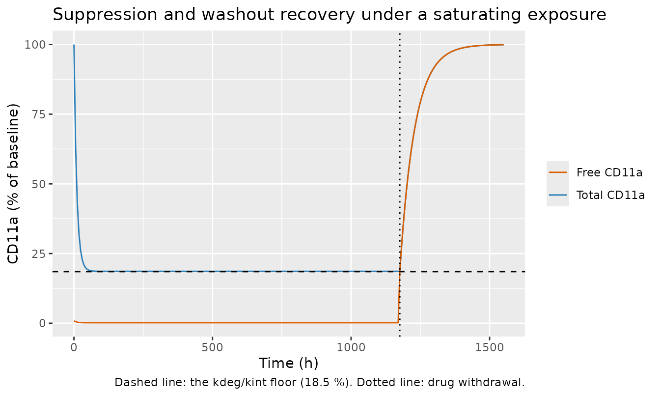
Comparison against Chetty 2014 Figure 3
Chetty 2014 Figure 3 plots CD11a as a percentage of baseline over the
Gottlieb 2002 escalating regimen. Reproducing it needs an efalizumab
exposure profile, which the un-extracted PBPK layer supplied in the
paper. Here it is supplied instead by
Stein_2018_efalizumab, an in-registry two-compartment
quasi-steady-state TMDD efalizumab PK model (Stein and Peletier 2018,
fitted to the Bauer 1999 data). Only its drug
concentration is used: its own target layer is not comparable,
because Stein and Peletier report ke(R) = ke(CR) = 4400 /day as
practically unidentifiable, giving a baseline target pool some 5000-fold
smaller than the Chetty 2014 Rmax.
ui_pk <- rxode2::rxode(readModelDb("Stein_2018_efalizumab"))

# Gottlieb 2002 escalating regimen; Stein 2018 uses days and nmol, with a
# 150 kDa antibody and a 70 kg subject (Stein and Peletier 2018 page 672).
dose_mgkg <- c(0.3, 0.4, 0.6, 1, 1, 1, 1)
tdose_h   <- (0:6) * 168
amt_nmol  <- dose_mgkg * 70 * 1e6 / 150000

ev_pk <- dplyr::bind_rows(
  data.frame(id = 1L, time = tdose_h / 24, evid = 1L, amt = amt_nmol, cmt = "central"),
  data.frame(id = 1L, time = seq(0, 1400, by = 6) / 24, evid = 0L,
             amt = NA_real_, cmt = "central")
) |> dplyr::arrange(time, dplyr::desc(evid))

# Stein 2018 reports total drug in nM; convert to ug/mL on the Chetty MW.
driver <- rxode2::rxSolve(ui_pk, ev_pk, returnType = "data.frame") |>
  dplyr::transmute(time_h = time * 24, cp_ugml = Cc * mw / 1e6)

stopifnot(nrow(driver) > 200, all(is.finite(driver$cp_ugml)),
          max(driver$cp_ugml) > 10, max(driver$cp_ugml) < 100)
range(driver$cp_ugml)
#> [1]  0.0472364 36.8949045
This driver runs roughly 1.5 to 2-fold above the profile Chetty 2014
predicts in its own Figure 2C (weekly peaks rising from about 5 to about
30 ug/mL, pre-dose troughs from about 0.5 to about 7 ug/mL). Both are
far above Km, which is what matters for the total pool.
ev_f3 <- data.frame(id = 1L, time = driver$time_h, evid = 0L, amt = NA_real_,
                    cmt = "total_target", CP_EFALIZUMAB_UGML = driver$cp_ugml)
s_f3 <- rxode2::rxSolve(rxode2::zeroRe(ui_cd11a), ev_f3,
                        returnType = "data.frame", covsInterpolation = "linear")
#> ℹ omega/sigma items treated as zero: 'etalkdeg'

# Digitised from Chetty 2014 Figure 3 (values read off the panel; no numeric
# annotations are printed, so these carry digitisation error of a few points).
fig3 <- tibble::tribble(
  ~time, ~observed_gottlieb, ~predicted_chetty,
      0,               100,                100,
    168,                29,                 24,
    336,              19.5,                 10,
    504,              20.5,                 10,
    672,                24,                 18,
    864,                25,                  9,
   1008,                28,                 14,
   1344,                31,                 52
)

fig3_cmp <- fig3 |>
  dplyr::left_join(
    s_f3 |> dplyr::select(time, model_total = pctTotalCd11a,
                          model_free = pctFreeCd11a),
    by = "time"
  )

fig3_cmp |>
  dplyr::rename(
    "Time (h)"                    = time,
    "Observed, Gottlieb 2002"     = observed_gottlieb,
    "Predicted, Chetty Figure 3"  = predicted_chetty,
    "This model, TOTAL CD11a"     = model_total,
    "This model, FREE CD11a"      = model_free
  ) |>
  knitr::kable(digits = 2,
caption = "CD11a as a percentage of baseline. The two source columns are digitised from Chetty 2014 Figure 3 and carry a few percentage points of reading error; the model columns are driven by the Stein 2018 plasma profile above.")| Time (h) | Observed, Gottlieb 2002 | Predicted, Chetty Figure 3 | This model, TOTAL CD11a | This model, FREE CD11a |
|---|---|---|---|---|
| 0 | 100.0 | 100 | 100.00 | 0.97 |
| 168 | 29.0 | 24 | 24.69 | 0.18 |
| 336 | 19.5 | 10 | 19.99 | 0.10 |
| 504 | 20.5 | 10 | 18.92 | 0.05 |
| 672 | 24.0 | 18 | 18.67 | 0.05 |
| 864 | 25.0 | 9 | 18.58 | 0.10 |
| 1008 | 28.0 | 14 | 18.61 | 0.04 |
| 1344 | 31.0 | 52 | 18.96 | 0.63 |
Two things follow, and they point in opposite directions.
The total pool tracks the observed data well for the first
three weeks. The model returns 24.7 % at 168 h against 29 %
observed (and against 24 % for Chetty’s own predicted series), 20.0 %
against 19.5 %, and 18.9 % against 20.5 %. That agreement is structural
rather than fitted: once the concentration is far above Km,
the total pool sits on its kdeg / kint floor whatever the
exposure. From 672 h onward the observed series drifts upward, to 31 %
by 1344 h, while the model stays pinned near 18.6 % – the total pool
cannot rise while drug is present.
The free pool is nowhere near Chetty’s predicted series. Driven by a plasma concentration, free CD11a falls to 0.04 to 1 % of baseline, one to two orders of magnitude below the 9 to 24 % of Figure 3. This is discussed under “Assumptions and deviations” below, together with the driver concentration the Figure 3 values imply.
dplyr::bind_rows(
  s_f3 |> dplyr::transmute(time, value = pctTotalCd11a, series = "Model: total CD11a"),
  s_f3 |> dplyr::transmute(time, value = pctFreeCd11a,  series = "Model: free CD11a")
) |>
  ggplot(aes(time, value, colour = series)) +
  geom_line() +
  geom_point(
    data = fig3 |>
      tidyr::pivot_longer(-time, names_to = "series", values_to = "value") |>
      dplyr::mutate(series = dplyr::recode(series,
        observed_gottlieb = "Digitised: Gottlieb 2002 observed",
        predicted_chetty  = "Digitised: Chetty Figure 3 predicted")),
    aes(time, value, colour = series), inherit.aes = FALSE, size = 2
  ) +
  scale_y_continuous(limits = c(0, 105)) +
  scale_colour_manual(values = c(
    "Model: total CD11a" = "#2c7fb8", "Model: free CD11a" = "#d95f02",
    "Digitised: Gottlieb 2002 observed" = "#1b7837",
    "Digitised: Chetty Figure 3 predicted" = "#762a83"), name = NULL) +
  theme(legend.position = "bottom") +
  guides(colour = guide_legend(nrow = 2)) +
  labs(x = "Time (h)", y = "CD11a (% of baseline)",
       title = "Replicates Figure 3 of Chetty 2014",
       caption = "Exposure driver from Stein_2018_efalizumab, not from the un-extracted Chetty PBPK layer.")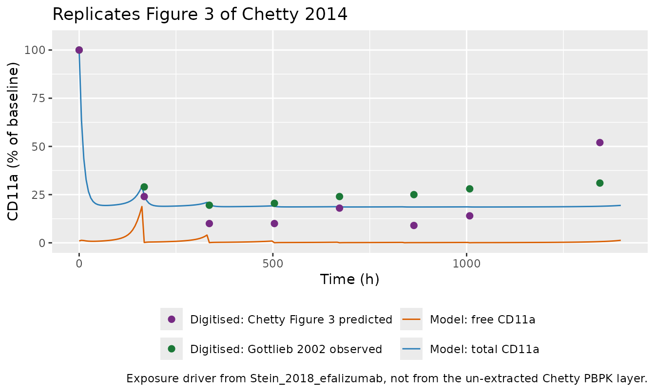
Between-subject variability
Chetty 2014 Table 1 attaches a CV to exactly two compound-file entries: CLiv (30 %), which belongs to the un-extracted PBPK layer, and Kdeg (10 %), which belongs here.
rxode2::rxSetSeed(20140670)
set.seed(20140670)

n_sub  <- 200L
grid_c <- seq(0, 1400, by = 12)
ev_coh <- do.call(rbind, lapply(seq_len(n_sub), function(i) {
  data.frame(id = i, time = grid_c, evid = 0L, amt = NA_real_,
             cmt = "total_target",
             CP_EFALIZUMAB_UGML = approx(driver$time_h, driver$cp_ugml,
                                         xout = grid_c, rule = 2)$y)
}))

s_coh <- rxode2::rxSolve(ui_cd11a, ev_coh, returnType = "data.frame",
                         covsInterpolation = "linear")

kdeg_i <- s_coh |> dplyr::group_by(id) |> dplyr::summarise(kdeg = dplyr::first(kdeg))
cv_kdeg <- sd(kdeg_i$kdeg) / mean(kdeg_i$kdeg)

# The sampled CV is a cohort statistic, so the bound is wide enough to hold for
# any cohort rxode2 can draw. Realised 9.82 / 9.92 / 10.33 / 10.76 % at 1 / 2 /
# 4 / 16 solver threads; n = 200 gives a standard error near 0.5 points on a
# 10 % CV. The 5-18 % bracket still goes red on a mis-transcribed CV (the next
# plausible mis-readings, 1 % and 30 %, both break it).
stopifnot(cv_kdeg > 0.05, cv_kdeg < 0.18)
c(target_cv = 0.10, realised_cv = cv_kdeg)
#>   target_cv realised_cv
#>  0.10000000  0.09821983
s_coh |>
  dplyr::group_by(time) |>
  dplyr::summarise(
    Q05 = quantile(pctTotalCd11a, 0.05),
    Q50 = quantile(pctTotalCd11a, 0.50),
    Q95 = quantile(pctTotalCd11a, 0.95),
    .groups = "drop"
  ) |>
  ggplot(aes(time, Q50)) +
  geom_ribbon(aes(ymin = Q05, ymax = Q95), alpha = 0.25) +
  geom_line() +
  labs(x = "Time (h)", y = "Total CD11a (% of baseline)",
       title = "Total CD11a with the published 10 % CV on Kdeg",
       caption = "Median and 5th-95th percentiles, 200 virtual subjects.")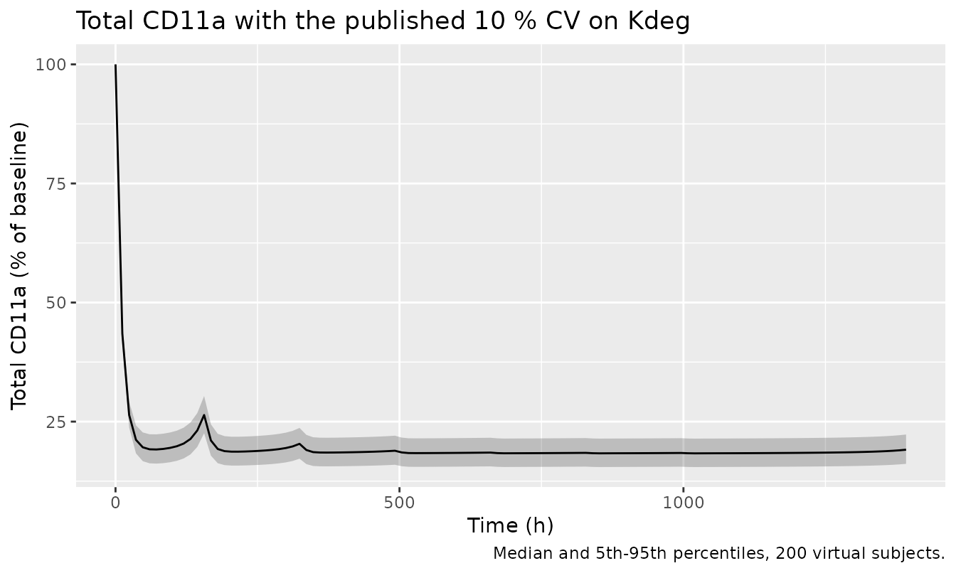
The band is narrow because the on-treatment plateau
kdeg / (kdeg + kint * f) is dominated by kint,
which the paper reports without variability.
Part 2: the PASI disease-progression model
Chetty 2014 prints the efficacy model as a closed form,
Y(t) = Yss + (Y(0) - Yss) * exp(-ln(2) / Tp * t),
with Y(0) and Yss read off the clinical
study being reproduced and Tp the paper’s only fitted
parameter, 397 h. The model file writes the equivalent indirect-response
balance d(pasi)/dt = kin - kout * pasi with
kout = ln(2)/Tp and kin = Yss * kout, using
the canonical turnover parameters; the first gate below confirms the two
forms agree.
ui_pasi_gordon <- ui_pasi |>
  rxode2::ini(lrbase = log(19), lkin = log(9.5 * log(2) / 397))
#> ℹ change initial estimate of `lrbase` to `2.94443897916644`
#> ℹ change initial estimate of `lkin` to `-4.09915740266236`

tp_h  <- 397
grid_p <- seq(0, 2100, by = 6)
ev_p <- data.frame(id = 1L, time = grid_p, evid = 0L, amt = NA_real_, cmt = "pasi")

s_gott <- rxode2::rxSolve(rxode2::zeroRe(ui_pasi),        ev_p, returnType = "data.frame")
#> ℹ omega/sigma items treated as zero: 'etalrbase', 'etalkin'
s_gord <- rxode2::rxSolve(rxode2::zeroRe(ui_pasi_gordon), ev_p, returnType = "data.frame")
#> ℹ omega/sigma items treated as zero: 'etalrbase', 'etalkin'
Gate 6: the ODE against the paper’s printed closed form
closed_form <- function(t, y0, yss) yss + (y0 - yss) * exp(-log(2) * t / tp_h)

err_gott <- max(abs(s_gott$pasi - closed_form(grid_p, 24.8, 14.8)) /
                  closed_form(grid_p, 24.8, 14.8))
err_gord <- max(abs(s_gord$pasi - closed_form(grid_p, 19.0,  9.5)) /
                  closed_form(grid_p, 19.0,  9.5))

stopifnot(err_gott < 1e-5, err_gord < 1e-5)
c(max_rel_error_gottlieb = err_gott, max_rel_error_gordon = err_gord)
#> max_rel_error_gottlieb   max_rel_error_gordon
#>           1.136562e-07           1.413623e-07
Gate 7: endpoints and the fitted progression half-life
pasi(0) must equal the published baseline, the asymptote
must equal the published Yss, and the time at which half
the total drop has occurred must equal the fitted Tp of 397
h. The Gordon cohort’s total improvement must also reproduce the paper’s
stated basis for choosing its asymptote: “a 1 mg/kg/week given by iv
infusion usually produces a change in PASI score from baseline of about
45-50 %”.
half_time <- function(s, y0, yss) {
  target <- (y0 + yss) / 2
  approx(s$pasi, s$time, xout = target)$y
}

drop_pct <- function(y0, yss) 100 * (y0 - yss) / y0

stopifnot(
  abs(s_gott$pasi[1] - 24.8) < 1e-10,
  abs(s_gord$pasi[1] - 19.0) < 1e-10,
  abs(s_gott$pasiSs[1] - 14.8) < 1e-10,
  abs(s_gord$pasiSs[1] -  9.5) < 1e-10,
  abs(half_time(s_gott, 24.8, 14.8) - tp_h) < 1,
  abs(half_time(s_gord, 19.0,  9.5) - tp_h) < 1,
  drop_pct(19.0, 9.5) >= 44, drop_pct(19.0, 9.5) <= 51
)

tibble::tibble(
  Cohort            = c("Gottlieb 2002 (escalating)", "Gordon 2003 (1 mg/kg/week)"),
  `Y(0)`            = c(s_gott$pasi[1], s_gord$pasi[1]),
  `Yss`             = c(s_gott$pasiSs[1], s_gord$pasiSs[1]),
  `Total drop (%)`  = c(drop_pct(24.8, 14.8), drop_pct(19.0, 9.5)),
  `t to half drop (h)` = c(half_time(s_gott, 24.8, 14.8), half_time(s_gord, 19.0, 9.5))
) |>
  knitr::kable(digits = 3,
caption = "PASI endpoints. The time to half the total drop recovers the fitted Tp of 397 h by construction; the Gordon total drop of 50.0 % reproduces the paper's stated 45-50 % basis for setting Yss = 9.5.")| Cohort | Y(0) | Yss | Total drop (%) | t to half drop (h) |
|---|---|---|---|---|
| Gottlieb 2002 (escalating) | 24.8 | 14.8 | 40.323 | 397.004 |
| Gordon 2003 (1 mg/kg/week) | 19.0 | 9.5 | 50.000 | 397.004 |
Comparison against Chetty 2014 Figure 4
# Digitised from Chetty 2014 Figure 4 (observed squares, upper panel; observed
# circles, lower panel). Assessment times are the nominal weekly / two-weekly
# schedules of the two studies. Digitisation error of roughly +/- 0.5 PASI
# units should be assumed.
fig4_gott <- tibble::tibble(
  time     = c(0, 168, 336, 504, 672, 840, 1008, 1344),
  observed = c(24.8, 23.5, 21.1, 17.8, 15.8, 13.7, 13.7, 13.0)
)
fig4_gord <- tibble::tibble(
  time     = c(0, 336, 672, 1008, 1344, 1680, 2016),
  observed = c(19.0, 17.2, 14.8, 12.6, 10.8, 9.75, 9.0)
)

cmp4 <- dplyr::bind_rows(
  fig4_gott |> dplyr::mutate(cohort = "Gottlieb 2002 (escalating)",
                             model = closed_form(time, 24.8, 14.8)),
  fig4_gord |> dplyr::mutate(cohort = "Gordon 2003 (1 mg/kg/week)",
                             model = closed_form(time, 19.0, 9.5))
) |>
  dplyr::mutate(pct_diff = 100 * (model - observed) / observed)

cmp4 |>
  dplyr::rename("Cohort" = cohort, "Time (h)" = time,
                "Observed PASI (digitised)" = observed,
                "Model PASI" = model, "Difference (%)" = pct_diff) |>
  dplyr::relocate(Cohort) |>
  knitr::kable(digits = 2,
caption = "Extracted PASI model against the observed points of Chetty 2014 Figure 4. Not used as a pass/fail gate: the observed values are digitised, and the systematic tail bias is a real property of the printed equation (see below).")| Cohort | Time (h) | Observed PASI (digitised) | Model PASI | Difference (%) |
|---|---|---|---|---|
| Gottlieb 2002 (escalating) | 0 | 24.80 | 24.80 | 0.00 |
| Gottlieb 2002 (escalating) | 168 | 23.50 | 22.26 | -5.29 |
| Gottlieb 2002 (escalating) | 336 | 21.10 | 20.36 | -3.50 |
| Gottlieb 2002 (escalating) | 504 | 17.80 | 18.95 | 6.45 |
| Gottlieb 2002 (escalating) | 672 | 15.80 | 17.89 | 13.25 |
| Gottlieb 2002 (escalating) | 840 | 13.70 | 17.11 | 24.87 |
| Gottlieb 2002 (escalating) | 1008 | 13.70 | 16.52 | 20.59 |
| Gottlieb 2002 (escalating) | 1344 | 13.00 | 15.76 | 21.21 |
| Gordon 2003 (1 mg/kg/week) | 0 | 19.00 | 19.00 | 0.00 |
| Gordon 2003 (1 mg/kg/week) | 336 | 17.20 | 14.78 | -14.05 |
| Gordon 2003 (1 mg/kg/week) | 672 | 14.80 | 12.44 | -15.95 |
| Gordon 2003 (1 mg/kg/week) | 1008 | 12.60 | 11.13 | -11.63 |
| Gordon 2003 (1 mg/kg/week) | 1344 | 10.80 | 10.41 | -3.62 |
| Gordon 2003 (1 mg/kg/week) | 1680 | 9.75 | 10.01 | 2.62 |
| Gordon 2003 (1 mg/kg/week) | 2016 | 9.00 | 9.78 | 8.68 |
sim4 <- dplyr::bind_rows(
  s_gott |> dplyr::transmute(time, pasi, cohort = "Gottlieb 2002 (escalating)"),
  s_gord |> dplyr::transmute(time, pasi, cohort = "Gordon 2003 (1 mg/kg/week)")
)

ggplot(sim4, aes(time, pasi)) +
  geom_line(colour = "#2c7fb8") +
  geom_point(data = dplyr::bind_rows(
    fig4_gott |> dplyr::mutate(cohort = "Gottlieb 2002 (escalating)"),
    fig4_gord |> dplyr::mutate(cohort = "Gordon 2003 (1 mg/kg/week)")
  ), aes(time, observed), size = 2, colour = "#1b7837") +
  facet_wrap(~cohort) +
  expand_limits(y = 0) +
  labs(x = "Time (h)", y = "PASI score",
       title = "Replicates Figure 4 of Chetty 2014",
       caption = "Line: extracted model. Points: observed PASI digitised from Figure 4.")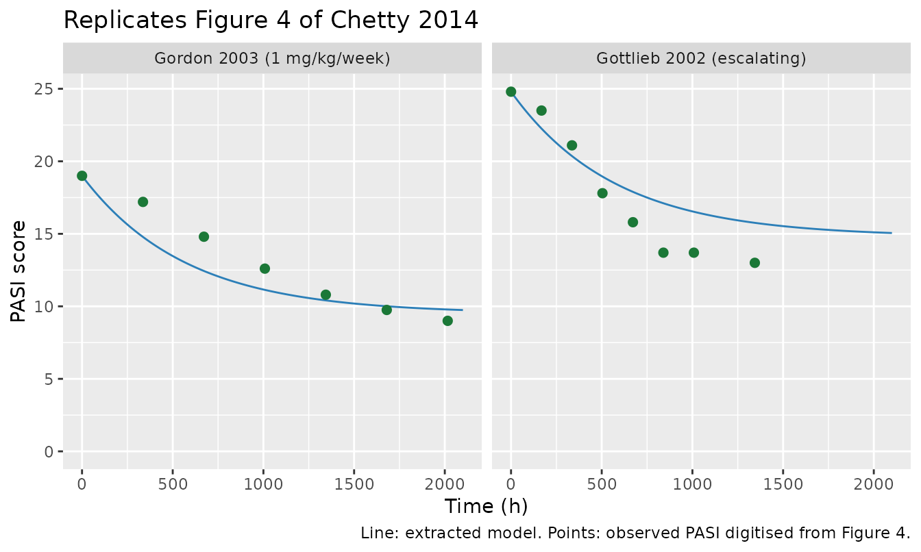
The model reproduces the observed decline closely over the first
three weeks in both cohorts and then sits systematically above the
observed points, by up to about 25 % in the Gottlieb cohort and about 15
% in the Gordon cohort. That bias is inherent to the printed equation:
over the 1176 h treatment period, which is only three progression
half-lives, an exponential retains 12.5 % of the initial gap, so the
model cannot reach Yss within the observation window. See
below.
Between-subject variability
Chetty 2014 reports a CV alongside each cohort input it took from
Gottlieb 2002: 10.8 % on the baseline score and 22 % on the asymptote.
Because kout is fixed, the variance placed on
kin transfers unchanged to
Yss = kin / kout.
rxode2::rxSetSeed(20140670)
set.seed(20140670)

ev_pcoh <- do.call(rbind, lapply(seq_len(200L), function(i) {
  data.frame(id = i, time = seq(0, 1400, by = 12), evid = 0L,
             amt = NA_real_, cmt = "pasi")
}))
s_pcoh <- rxode2::rxSolve(ui_pasi, ev_pcoh, returnType = "data.frame")

per_sub <- s_pcoh |>
  dplyr::group_by(id) |>
  dplyr::summarise(base = dplyr::first(pasi), yss = dplyr::first(pasiSs),
                   .groups = "drop")
cv_base <- sd(per_sub$base) / mean(per_sub$base)
cv_yss  <- sd(per_sub$yss)  / mean(per_sub$yss)

# Cohort statistics: bounds are wide enough to hold for any cohort rxode2 can
# draw at n = 200 (standard error near 0.5 and 1.1 points respectively).
# Realised baseline CV 10.61 / 10.70 / 11.15 / 11.63 % and asymptote CV
# 22.23 / 22.15 / 22.32 / 23.10 % at 1 / 2 / 4 / 16 solver threads. Both
# brackets still go red on a mis-transcribed CV.
stopifnot(cv_base > 0.06, cv_base < 0.18,
          cv_yss  > 0.12, cv_yss  < 0.35)
c(target_cv_baseline = 0.108, realised_cv_baseline = cv_base,
  target_cv_yss = 0.22, realised_cv_yss = cv_yss)
#>   target_cv_baseline realised_cv_baseline        target_cv_yss
#>            0.1080000            0.1060864            0.2200000
#>      realised_cv_yss
#>            0.2222860
s_pcoh |>
  dplyr::group_by(time) |>
  dplyr::summarise(
    Q05 = quantile(pasi, 0.05), Q50 = quantile(pasi, 0.50),
    Q95 = quantile(pasi, 0.95), .groups = "drop"
  ) |>
  ggplot(aes(time, Q50)) +
  geom_ribbon(aes(ymin = Q05, ymax = Q95), alpha = 0.25) +
  geom_line() +
  geom_point(data = fig4_gott, aes(time, observed), colour = "#1b7837", size = 2) +
  expand_limits(y = 0) +
  labs(x = "Time (h)", y = "PASI score",
       title = "PASI with the published CVs on the baseline and the asymptote",
       caption = "Median and 5th-95th percentiles, 200 virtual subjects; points are the digitised Gottlieb 2002 observations.")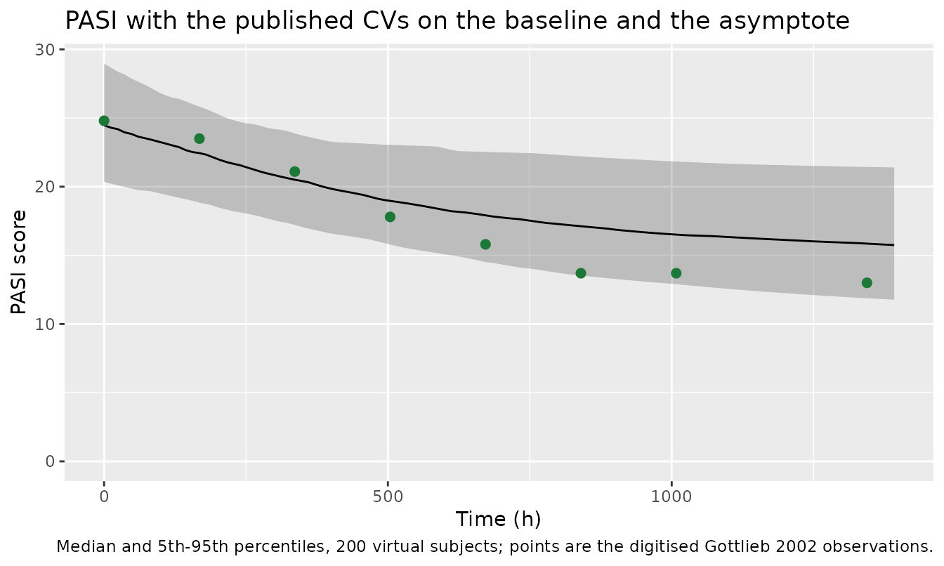
Assumptions and deviations
The PBPK layer is not extracted. Chetty 2014 Table 1
publishes no volume term of any kind; the Mechanistic FcRn structure and
all of its physiology are Simcyp database outputs. Consequently this
vignette cannot reproduce Figure 2 (concentration-time profiles) or
Table 2 (predicted versus observed clearance), and the exposure driver
used for the Figure 3 comparison comes from
Stein_2018_efalizumab, a different publication, not from
Chetty’s own PBPK model. Its profile runs roughly 1.5 to 2-fold above
Chetty’s Figure 2C.
The two extracted layers are not coupled, because the
coupling constant is unpublished. Chetty 2014 Methods states
that the PASI baseline Y(0) is “modulated in proportion to
concentration of bound CD11a”, and the Discussion repeats that
“efalizumab modulates the baseline PASI score, i.e., Y(0)”. No
proportionality constant, functional form or linking equation is given
anywhere in the paper, and the paper itself supplies both
Y(0) and Yss as inputs read off the clinical
study being reproduced – for the Gordon cohort it sets
Yss = 9.5 from the prior expectation that “a 1 mg/kg/week
given by iv infusion usually produces a change in PASI score from
baseline of about 45-50 %”, not from any simulated CD11a trajectory. The
PASI model is therefore packaged as an on-treatment time course whose
magnitude of benefit is a user input, which is exactly how the paper
applied it. Nothing has been invented to bridge the two.
Which matrix drives CD11a binding is not stated, and it
matters enormously for the free pool. Driven by a plasma
concentration, this model predicts free CD11a at 0.04 to 1 % of baseline
over the escalating regimen, against the 9 to 24 % of Chetty’s Figure 3.
The discrepancy is not a transcription error: the free-pool relation
1 / (1 + (kint / (kdeg * Km)) * C) falls to half at
C = kdeg * Km / kint, which with the Table 1 values is
0.016 ug/mL – three orders of magnitude below therapeutic plasma
concentrations. Inverting the relation on the Figure 3 values gives the
driver those values imply:
backsolve_ugml <- function(pct) (kdeg * km / kint) * (100 / pct - 1) * mw / 1000

tibble::tibble(
  `Chetty Figure 3 predicted free CD11a (%)` = c(24, 18, 14, 10, 9),
  `Implied driver (ug/mL)` = backsolve_ugml(c(24, 18, 14, 10, 9))
) |>
  knitr::kable(digits = 4,
caption = "Efalizumab concentration implied by each of Chetty's own Figure 3 predicted free-CD11a values, obtained by inverting the closed form. Compare with the 0.5 to 30 ug/mL plasma range of the paper's Figure 2C.")| Chetty Figure 3 predicted free CD11a (%) | Implied driver (ug/mL) |
|---|---|
| 24 | 0.0500 |
| 18 | 0.0719 |
| 14 | 0.0969 |
| 10 | 0.1420 |
| 9 | 0.1595 |
Those implied concentrations, 0.05 to 0.16 ug/mL, are one to two
orders of magnitude below the plasma profile of the paper’s own Figure
2C. The most likely explanation is that the Simcyp implementation drove
target binding from a tissue interstitial concentration rather than from
plasma: Chetty 2014’s Introduction notes exactly this capability, that
“input to the PD model can be done from a tissue interstitial
compartment and not just from plasma, which is important when modeling
membrane bound receptors”. That interstitial concentration is an
internal output of the un-extracted PBPK layer, so it cannot be
reconstructed here. Users must decide which matrix their
CP_EFALIZUMAB_UGML trajectory represents; the total pool,
which saturates at kdeg / kint for any driver well above
Km, is largely insensitive to that decision, while the free
pool is not.
Chetty’s Figure 3 predicted series is not reproducible as either pool. It is non-monotone (24, 10, 10, 18, 9, 14 % at successive assessments while drug is present and accumulating) and five of its seven on-treatment points fall below 18.5 %, the total-pool floor implied by the paper’s own Table 1. No concentration trajectory can drive the total pool below that floor, and no single trajectory produces that ordering in the free pool either. The digitisation carries a few percentage points of error, which does not account for the pattern. The model’s total pool does track the Gottlieb 2002 observed series well over the first three weeks (24.7 versus 29 %, 20.0 versus 19.5 %, 18.9 versus 20.5 %) before the observed series drifts upward and the model stays on its floor.
The printed PASI equation and the paper’s own Figure 4 curves
disagree in the tail. The Figure 4 predicted curves fall
below their stated asymptotes late in the time course, reaching
about 13.9 against Yss = 14.8 in the Gottlieb panel and
about 8.7 against Yss = 9.5 in the Gordon panel, and they
step discontinuously upward at the weekly dose escalations of
the Gottlieb regimen. A first-order approach to a fixed asymptote can do
neither: it is monotone and cannot overshoot. Both features are
consistent with the unquantified CD11a-to-Y(0) modulation
being active in the Simcyp implementation but absent from the printed
equation. The printed equation tracks the paper’s own predicted curves
to within about 5 % over the first 1000 h and drifts to roughly 12 to 14
% by the end of follow-up.
No residual error is encoded. Chetty 2014 is a
simulation study and reports no residual-error model or assay
variability for either CD11a or PASI, so
propSd_total_target and propSd_pasi are
fixed(0) rather than invented.
Unit corrections and interpretations.
Kint is printed in Table 1 as 0.1 l/h and is
read as 0.1 1/h per the Figure 1 legend; this is the only value in
either file whose units were corrected. Km is labelled a
“rate constant” in Table 1 but printed and used as a concentration, per
the Methods definition. Ksyn and Kdeg have
their orders transposed between Table 1 and the Figure 1 legend; Table 1
is dimensionally self-consistent and is taken as authoritative. See the
dimensional-analysis section above.
Distributional assumptions for the published CVs.
Chetty 2014 reports a CV % for Kdeg (10 %), the PASI
baseline (10.8 %) and the PASI asymptote (22 %), but does not state
which distribution family the Simcyp compound file and PD model sampled
from. All three are encoded as log-normal with
omega^2 = log(1 + CV^2), the library convention for a
reported CV on a strictly positive quantity. No CV is published for
Kint, Km, Rmax or
Tp, so those carry no variability – consistent with the
Discussion’s own caveat that disease-progression variability “could not
be accurately assessed”.
No NCA validation. Both extracted layers are mechanistic PD models with no dosing events and no concentration output, so PKNCA is not the appropriate check; the closed-form, mass-balance, steady-state and washout gates above replace it, per the endogenous-model validation pattern. The only NCA-style quantity the paper reports, the clearance table (Table 2), belongs to the un-extracted PBPK layer.
Digitised values. The Figure 3 and Figure 4
comparison points in this vignette were read off the published panels;
neither figure prints numeric annotations. They are used for display and
for the deviation discussion only, never as the source of a parameter
value and never as a pass/fail gate. Every stopifnot()
above is anchored either on a closed-form identity that shares its
parameters with the model or on a value the paper prints in text.