Piperacillin, total and unbound, in perioperative critically ill children (Tan 2025)
Source:vignettes/articles/Tan_2025_piperacillin.Rmd
Tan_2025_piperacillin.RmdModel and source
- Citation: Tan WR, Irie K, McIntire C, Torres JL, Jones R, Gibson A, Mizuno T, Tang Girdwood S. Model-informed dose optimization for prophylactic piperacillin-tazobactam in perioperative pediatric critically ill patients. Antimicrob Agents Chemother. 2025;69(3):e01227-24. doi:10.1128/aac.01227-24
- Total piperacillin: Two-compartment IV population PK model for TOTAL plasma piperacillin (given as piperacillin-tazobactam) in critically ill children receiving perioperative prophylaxis (Tan 2025), with allometric body-weight scaling, a bedside-Schwartz creatinine-clearance power effect on CL, and inter-occasion variability on CL for the pre- and post-operative periods (the intraoperative period is the zero-IOV reference). The paper’s unbound-piperacillin fit is Tan_2025_piperacillin_unbound.
- Unbound piperacillin: Two-compartment IV population PK model for UNBOUND (free) plasma piperacillin (given as piperacillin-tazobactam) in critically ill children receiving perioperative prophylaxis (Tan 2025), with allometric body-weight scaling, a bedside-Schwartz creatinine-clearance power effect on CL, and inter-occasion variability on CL for the pre- and post-operative periods (the intraoperative period is the zero-IOV reference). This is the model the paper used for all of its dosing simulations; the paper’s total-piperacillin fit is Tan_2025_piperacillin_total.
- Article: https://doi.org/10.1128/aac.01227-24 (open access; supplementary Tables S1-S2 and Figures S1-S9 in the article’s supplemental material)
Tan 2025 fitted total and unbound (free) piperacillin concentrations from the same samples as two separate population PK models with the same structure: two compartments, allometric body-weight scaling to 70 kg, a bedside-Schwartz creatinine clearance (CrCL) power effect on clearance, and inter-occasion variability (IOV) on clearance for the pre- and post-operative periods. The paper treats the total model as its primary analysis (Table 2) and uses the unbound model (Table S2) for every dosing simulation. Both are packaged here.
Population
Thirty-four critically ill children in the paediatric intensive care unit of Cincinnati Children’s Hospital Medical Center who received prophylactic piperacillin-tazobactam every 2-3 h around surgery (Table 1): median age 7.07 years (IQR 3.05-14.48), median weight 20.0 kg (IQR 12.65-55.33), 55.9% female, median baseline bedside-Schwartz CrCL 143 mL/min/1.73 m^2 (IQR 102.81-181.53). Surgeries were liver transplantation (44.1%), total pancreatectomy with islet auto-transplantation (5.9%), non-transplant abdominal surgery (26.5%) and ear-nose-throat surgery (23.5%); median surgery duration 5.32 h. Patients under 45 kg received 80-90 mg/kg piperacillin and patients over 45 kg 3000 or 4000 mg, as 30-min infusions. Scavenged opportunistic sampling gave 286 total and 285 unbound concentrations (1-19 per patient).
The same information is available programmatically via
readModelDb("Tan_2025_piperacillin_unbound")()$population.
Source trace
Both model files carry the per-parameter origin as an in-file comment. Values for the total model come from Table 2 and for the unbound model from Table S2.
| Equation / parameter | Total (Table 2) | Unbound (Table S2) | Source location |
|---|---|---|---|
lcl (CL, L/h/70 kg) |
log(7.1) | log(8.95) | Table 2 / Table S2 |
lvc (V1, L/70 kg) |
log(17.2) | log(22.4) | Table 2 / Table S2 |
lq (Q, L/h/70 kg) |
log(3.25) | log(2.51) | Table 2 / Table S2 |
lvp (V2, L/70 kg) |
log(4.79) | log(4.48) | Table 2 / Table S2 |
e_crcl_cl (CrCL exponent on CL) |
0.484 | 0.457 | Table 2 / Table S2 |
e_wt_cl, e_wt_vc (allometric
exponents) |
0.75, 1 fixed | 0.75, 1 fixed | Methods, ‘Population PK modeling’; Table S1 footnote 1 |
etalcl (IIV CL) |
28.7% CV -> 0.07915 | 27.1% CV -> 0.07087 | Table 2 / Table S2, omega^2 = log(1 + CV^2) |
etalvc (IIV V1) |
41% CV -> 0.15538 | 37.5% CV -> 0.13158 | Table 2 / Table S2 |
etaiov_cl_1 (IOV CL, preoperative) |
37.7% CV -> 0.13289 | 50.7% CV -> 0.22877 | Table 2 / Table S2 |
etaiov_cl_3 (IOV CL, postoperative) |
33.5% CV -> 0.10636 | 44.4% CV -> 0.17993 | Table 2 / Table S2 |
propSd (proportional residual error) |
0.371 | 0.427 | Table 2 / Table S2 |
| CL = CL_pop (WT/70)^0.75 (CrCL/120)^theta | Results, final CL equation; Methods covariate equations | ||
| No IOV in the intraoperative period | Methods, IOV equation and text | ||
| IIV on Q and V2 fixed to 0 | Results, ‘Population PK modeling’ | ||
| Two-compartment, first-order elimination, IV infusion | Methods; Results |
Typical-value check against the paper’s simulations
The unbound model’s typical clearance for the Figure 3 patient (20
kg, CrCL 143 mL/min/1.73 m^2) is
8.95 * (20/70)^0.75 * (143/120)^0.457 L/h. A continuous
infusion at steady state gives Css = rate / CL, and the
medians that Figure 3 prints for its two continuous-infusion panels
(read off the figure by the maintainers: about 14.5 mg/L for 2.75
mg/kg/h and about 48.5 mg/L for 9.25 mg/kg/h) follow from it directly.
This checks the CL, the allometric scaling and the CrCL term of the
packaged unbound model against the authors’ own simulation, without
random effects.
mod_free <- readModelDb("Tan_2025_piperacillin_unbound")
mod_tot <- readModelDb("Tan_2025_piperacillin_total")

ini_free <- rxode2::rxode(mod_free)$theta
#> ℹ parameter labels from comments will be replaced by 'label()'
#> Warning: some etas defaulted to non-mu referenced, possible parsing error: etaiov_cl_1, etaiov_cl_3
#> as a work-around try putting the mu-referenced expression on a simple line
cl_typ <- exp(ini_free[["lcl"]]) * (20 / 70)^0.75 * (143 / 120)^ini_free[["e_crcl_cl"]]

css_check <- tibble::tibble(
  regimen = c("10 mg/kg LD + 2.75 mg/kg/h", "20 mg/kg LD + 9.25 mg/kg/h"),
  rate_mg_h = c(2.75, 9.25) * 20,
  css_model = rate_mg_h / cl_typ,
  css_figure3 = c(14.5, 48.5)
) |>
  mutate(pct_diff = 100 * (css_model - css_figure3) / css_figure3)

css_check |>
  dplyr::rename(
    "Regimen" = regimen,
    "Infusion rate (mg/h)" = rate_mg_h,
    "Model Css (mg/L)" = css_model,
    "Figure 3 median (mg/L)" = css_figure3,
    "Difference (%)" = pct_diff
  ) |>
knitr::kable(digits = 2)| Regimen | Infusion rate (mg/h) | Model Css (mg/L) | Figure 3 median (mg/L) | Difference (%) |
|---|---|---|---|---|
| 10 mg/kg LD + 2.75 mg/kg/h | 55 | 14.51 | 14.5 | 0.10 |
| 20 mg/kg LD + 9.25 mg/kg/h | 185 | 48.82 | 48.5 | 0.66 |
Replicate Figure 3
Figure 3 simulates 1,000 virtual 20-kg patients with CrCL 143 mL/min/1.73 m^2 in the intraoperative period, which carries no IOV, under four regimens: 15 mg/kg and 55 mg/kg every 2 h as 30-min infusions, and a 10 or 20 mg/kg 30-min loading dose followed immediately by a 2.75 or 9.25 mg/kg/h continuous infusion. The bands are reproduced here with 200 virtual patients per regimen and without residual error; the paper’s continuous-infusion 5th-95th percentile bands (about 9.5-23 mg/L and 32-77 mg/L at steady state) match the spread that between-subject variability on CL alone produces, so residual error was evidently not added to the plotted bands.
rxode2::rxSetSeed(20250303)
n_per_arm <- 200
wt_fig <- 20
crcl_fig <- 143

regimens <- tibble::tribble(
  ~regimen,                                ~type, ~dose_mgkg, ~rate_mgkgh,
  "Q2H 15 mg/kg (1x MIC)",                 "q2h", 15,         NA,
  "LD 10 mg/kg + CI 2.75 mg/kg/h (1x MIC)", "ci",  10,         2.75,
  "Q2H 55 mg/kg (4x MIC)",                 "q2h", 55,         NA,
  "LD 20 mg/kg + CI 9.25 mg/kg/h (4x MIC)", "ci",  20,         9.25
) |>
  mutate(regimen = factor(regimen, levels = regimen))

fig3_times <- sort(unique(round(c(seq(0, 24, by = 0.1), seq(0.5, 24, by = 2)), 2)))

make_events <- function(reg_row, ids, wt, crcl, times, t_end = max(times)) {
  dose_mg <- reg_row$dose_mgkg * wt
  if (reg_row$type == "q2h") {
    dosing <- tidyr::expand_grid(id = ids, time = seq(0, t_end - 2, by = 2)) |>
      mutate(amt = dose_mg[match(id, ids)], rate = amt / 0.5)
  } else {
    ld <- tibble::tibble(id = ids, time = 0, amt = dose_mg, rate = amt / 0.5)
    ci_rate <- reg_row$rate_mgkgh * wt
    ci <- tibble::tibble(id = ids, time = 0.5, rate = ci_rate, amt = ci_rate * (t_end - 0.5))
    dosing <- bind_rows(ld, ci)
  }
  dosing <- dosing |> mutate(evid = 1L, cmt = "central")
  obs <- tidyr::expand_grid(id = ids, time = times) |>
    mutate(evid = 0L, amt = 0, rate = 0, cmt = "central")
  bind_rows(dosing, obs) |>
    left_join(tibble::tibble(id = ids, WT = wt, CRCL = crcl), by = "id") |>
    mutate(OCC = 2L, regimen = as.character(reg_row$regimen)) |>
    arrange(id, time, desc(evid))
}

ev_fig3 <- bind_rows(lapply(seq_len(nrow(regimens)), function(i) {
  ids <- (i - 1) * n_per_arm + seq_len(n_per_arm)
  make_events(regimens[i, ], ids, rep(wt_fig, n_per_arm), rep(crcl_fig, n_per_arm), times = fig3_times)
}))

sim_fig3 <- rxode2::rxSolve(mod_free, events = ev_fig3, keep = "regimen", returnType = "data.frame")
#> ℹ parameter labels from comments will be replaced by 'label()'
#> Warning: some etas defaulted to non-mu referenced, possible parsing error: etaiov_cl_1, etaiov_cl_3
#> as a work-around try putting the mu-referenced expression on a simple line

band_fig3 <- sim_fig3 |>
  group_by(regimen, time) |>
  summarise(
    p05 = quantile(Cc, 0.05), p50 = median(Cc), p95 = quantile(Cc, 0.95),
    .groups = "drop"
  )
targets <- tibble::tibble(
  regimen = factor(levels(regimens$regimen), levels = levels(regimens$regimen)),
  target = c(8, 8, 32, 32)
)
ggplot(band_fig3, aes(time)) +
  geom_ribbon(aes(ymin = p05, ymax = p95), fill = "grey70") +
  geom_line(aes(y = p50), linewidth = 0.8) +
  geom_hline(data = targets, aes(yintercept = target), colour = "red", linetype = "dashed") +
  facet_wrap(~regimen, scales = "free_y") +
  labs(x = "Time (h)", y = "Unbound piperacillin (mg/L)") +
  theme_bw()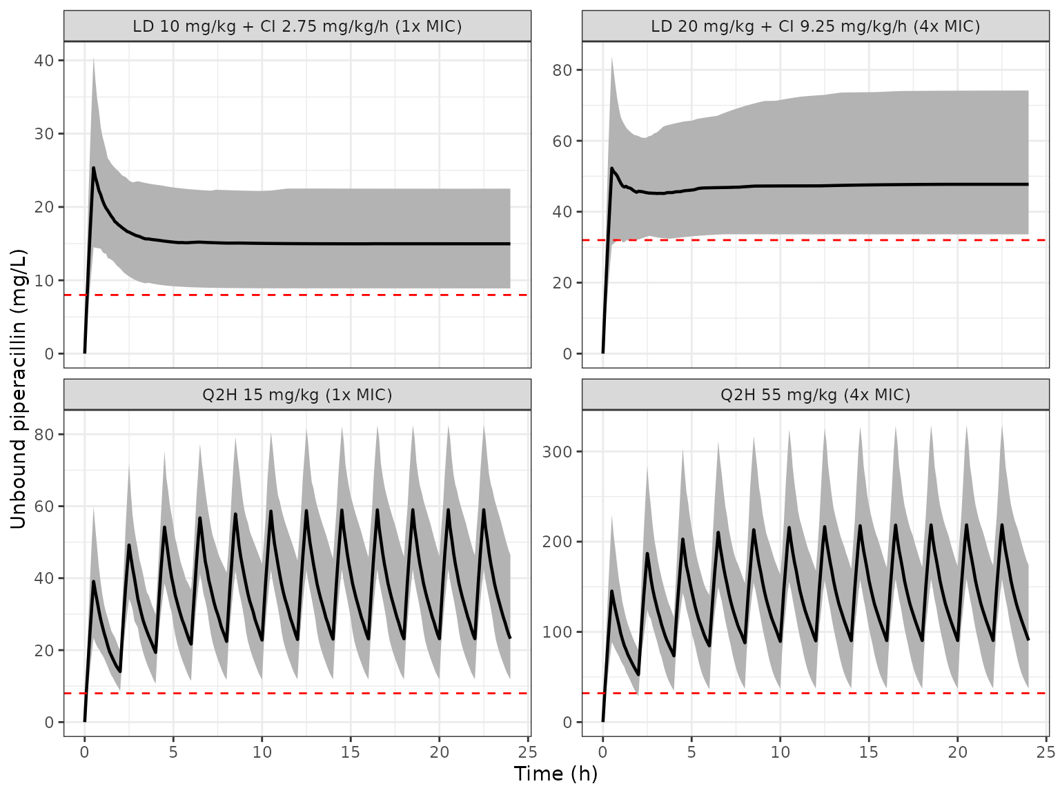
Replicates Figure 3 of Tan 2025: simulated unbound piperacillin in 20-kg patients with CrCL 143 mL/min/1.73 m^2. Black line, median; shaded band, 5th-95th percentiles; dashed red line, the 8 mg/L (1x MIC) or 32 mg/L (4x MIC) target.
The maintainers read the medians and band edges below off Figure 3. They are compared with the simulated medians at the same times; the first-dose trough of the 15 mg/kg regimen, the steady-state peak and trough of both Q2H regimens, and the steady-state plateau of both infusions are all reproduced.
fig3_digitised <- tibble::tribble(
  ~regimen,                                ~time, ~what,                       ~fig3,
  "Q2H 15 mg/kg (1x MIC)",                 0.5,   "first peak",                38.5,
  "Q2H 15 mg/kg (1x MIC)",                 2,     "first trough",              14,
  "Q2H 15 mg/kg (1x MIC)",                 22.5,  "steady-state peak",         59.5,
  "Q2H 15 mg/kg (1x MIC)",                 24,    "steady-state trough",       25,
  "Q2H 55 mg/kg (4x MIC)",                 0.5,   "first peak",                140,
  "Q2H 55 mg/kg (4x MIC)",                 22.5,  "steady-state peak",         219,
  "Q2H 55 mg/kg (4x MIC)",                 24,    "steady-state trough",       91,
  "LD 10 mg/kg + CI 2.75 mg/kg/h (1x MIC)", 0.5,   "end of loading dose",       25.5,
  "LD 10 mg/kg + CI 2.75 mg/kg/h (1x MIC)", 24,    "plateau",                   14.5,
  "LD 20 mg/kg + CI 9.25 mg/kg/h (4x MIC)", 0.5,   "end of loading dose",       51,
  "LD 20 mg/kg + CI 9.25 mg/kg/h (4x MIC)", 24,    "plateau",                   48.5
)

fig3_cmp <- fig3_digitised |>
  left_join(
    band_fig3 |> mutate(regimen = as.character(regimen), time = round(time, 2)),
    by = c("regimen", "time")
  ) |>
  mutate(pct_diff = 100 * (p50 - fig3) / fig3)

fig3_cmp |>
  select(regimen, what, time, fig3, p50, pct_diff) |>
  dplyr::rename(
    "Regimen" = regimen, "Point" = what, "Time (h)" = time,
    "Figure 3 median (mg/L)" = fig3, "Simulated median (mg/L)" = p50,
    "Difference (%)" = pct_diff
  ) |>
knitr::kable(digits = 1)| Regimen | Point | Time (h) | Figure 3 median (mg/L) | Simulated median (mg/L) | Difference (%) |
|---|---|---|---|---|---|
| Q2H 15 mg/kg (1x MIC) | first peak | 0.5 | 38.5 | 39.1 | 1.6 |
| Q2H 15 mg/kg (1x MIC) | first trough | 2.0 | 14.0 | 14.0 | 0.3 |
| Q2H 15 mg/kg (1x MIC) | steady-state peak | 22.5 | 59.5 | 59.0 | -0.8 |
| Q2H 15 mg/kg (1x MIC) | steady-state trough | 24.0 | 25.0 | 23.2 | -7.3 |
| Q2H 55 mg/kg (4x MIC) | first peak | 0.5 | 140.0 | 145.2 | 3.7 |
| Q2H 55 mg/kg (4x MIC) | steady-state peak | 22.5 | 219.0 | 218.6 | -0.2 |
| Q2H 55 mg/kg (4x MIC) | steady-state trough | 24.0 | 91.0 | 90.5 | -0.6 |
| LD 10 mg/kg + CI 2.75 mg/kg/h (1x MIC) | end of loading dose | 0.5 | 25.5 | 25.4 | -0.6 |
| LD 10 mg/kg + CI 2.75 mg/kg/h (1x MIC) | plateau | 24.0 | 14.5 | 15.0 | 3.3 |
| LD 20 mg/kg + CI 9.25 mg/kg/h (4x MIC) | end of loading dose | 0.5 | 51.0 | 52.3 | 2.5 |
| LD 20 mg/kg + CI 9.25 mg/kg/h (4x MIC) | plateau | 24.0 | 48.5 | 47.7 | -1.6 |
Replicate the Table 3 and Table 4 dosing recommendations
Tables 3 and 4 give, for each of five CrCL bands and four body-weight bands, the lowest dose at which more than 90% of virtual patients keep unbound piperacillin above the target (8 mg/L for 1x MIC, 32 mg/L for 4x MIC) for the whole intraoperative period. For Q2H dosing the criterion is the first trough (2 h); for continuous infusion it is the concentration over the surgery once the loading dose has been given. Covariates were drawn uniformly within each band (the open-ended bands as 70-89 kg and 130-159 mL/min/1.73 m^2, per the Methods). The continuous-infusion criterion is evaluated here as the minimum concentration from the end of the loading dose (0.5 h) to 8 h, which covers the cohort’s surgery durations (median 5.32 h, IQR 2.93-8.89).
wt_bands <- tibble::tribble(
  ~wt_band,   ~wt_lo, ~wt_hi,
  "10-29 kg", 10,     29,
  "30-49 kg", 30,     49,
  "50-69 kg", 50,     69,
  ">=70 kg",  70,     89
)
crcl_bands <- tibble::tribble(
  ~crcl_band, ~crcl_lo, ~crcl_hi,
  "20-29",    20,       29,
  "30-59",    30,       59,
  "60-89",    60,       89,
  "90-129",   90,       129,
  ">=130",    130,      159
)

# Table 3 (Q2H, mg/kg) and Table 4 (continuous infusion, mg/kg/h after a
# 10 or 20 mg/kg loading dose); rows CrCL band, columns weight band.
tab3_1x <- c(7.5, 7, 6.5, 6, 9, 8.5, 8, 7.5, 9.5, 9, 8.5, 8, 10.5, 10, 9.5, 9, 15, 11, 10.5, 10)
tab3_4x <- c(29, 27, 25, 25, 30, 30, 30, 30, 40, 38, 36, 34, 41, 39, 37, 35, 55, 45, 43, 41)
tab4_1x <- c(1.25, 1, 1, 1, 2, 2, 2, 2, 2, 2, 2, 2, 2.5, 2.25, 2.25, 2, 2.75, 2.5, 2.25, 2)
tab4_4x <- c(4.25, 4.25, 4.25, 3.25, 6, 6, 6, 6, 7.5, 6, 6, 6, 9, 7.5, 6, 6, 9.25, 7.75, 7.5, 6.5)

cells <- tidyr::expand_grid(crcl_band = crcl_bands$crcl_band, wt_band = wt_bands$wt_band) |>
  left_join(crcl_bands, by = "crcl_band") |>
  left_join(wt_bands, by = "wt_band")

recs <- bind_rows(
  cells |> mutate(target = 8, type = "q2h", dose_mgkg = tab3_1x, rate_mgkgh = NA_real_),
  cells |> mutate(target = 32, type = "q2h", dose_mgkg = tab3_4x, rate_mgkgh = NA_real_),
  cells |> mutate(target = 8, type = "ci", dose_mgkg = 10, rate_mgkgh = tab4_1x),
  cells |> mutate(target = 32, type = "ci", dose_mgkg = 20, rate_mgkgh = tab4_4x)
) |>
  mutate(cell = row_number(), regimen = as.character(cell))
nrow(recs)
#> [1] 80
rxode2::rxSetSeed(20250304)
n_cell <- 200
tab_times <- seq(0, 8, by = 0.25)

ev_tab <- bind_rows(lapply(seq_len(nrow(recs)), function(i) {
  r <- recs[i, ]
  ids <- (i - 1) * n_cell + seq_len(n_cell)
  make_events(
    r, ids,
    wt = stats::runif(n_cell, r$wt_lo, r$wt_hi),
    crcl = stats::runif(n_cell, r$crcl_lo, r$crcl_hi),
    times = tab_times
  ) |> mutate(cell = r$cell)
}))

sim_tab <- rxode2::rxSolve(mod_free, events = ev_tab, keep = "cell", returnType = "data.frame")
#> [====|====|====|====|====|====|====|====|====|====] 0:00:01

pta <- sim_tab |>
  left_join(recs |> select(cell, type, target), by = "cell") |>
  filter((type == "q2h" & abs(time - 2) < 1e-8) | (type == "ci" & time >= 0.5)) |>
  group_by(cell, id) |>
  summarise(cmin = min(Cc), target = first(target), .groups = "drop") |>
  group_by(cell) |>
  summarise(pta = 100 * mean(cmin > target), .groups = "drop") |>
  left_join(recs, by = "cell")
pta_wide <- pta |>
  mutate(
    criterion = paste0(ifelse(type == "q2h", "Q2H", "CI"), " ", ifelse(target == 8, "1x", "4x"), " MIC"),
    wt_band = factor(wt_band, levels = wt_bands$wt_band),
    crcl_band = factor(crcl_band, levels = crcl_bands$crcl_band)
  ) |>
  select(criterion, crcl_band, wt_band, pta) |>
  tidyr::pivot_wider(names_from = wt_band, values_from = pta) |>
  arrange(criterion, crcl_band)

pta_wide |>
  dplyr::rename("Criterion" = criterion, "CrCL (mL/min/1.73 m^2)" = crcl_band) |>
knitr::kable(digits = 0, caption = "Percentage of 200 virtual patients per cell meeting the target at the Table 3 / Table 4 recommended dose.")| Criterion | CrCL (mL/min/1.73 m^2) | 10-29 kg | 30-49 kg | 50-69 kg | >=70 kg |
|---|---|---|---|---|---|
| CI 1x MIC | 20-29 | 99 | 100 | 100 | 100 |
| CI 1x MIC | 30-59 | 100 | 100 | 100 | 100 |
| CI 1x MIC | 60-89 | 98 | 100 | 100 | 100 |
| CI 1x MIC | 90-129 | 97 | 100 | 100 | 100 |
| CI 1x MIC | >=130 | 96 | 100 | 100 | 99 |
| CI 4x MIC | 20-29 | 87 | 94 | 95 | 93 |
| CI 4x MIC | 30-59 | 93 | 94 | 96 | 96 |
| CI 4x MIC | 60-89 | 94 | 92 | 95 | 96 |
| CI 4x MIC | 90-129 | 87 | 92 | 92 | 89 |
| CI 4x MIC | >=130 | 89 | 90 | 91 | 92 |
| Q2H 1x MIC | 20-29 | 98 | 99 | 98 | 94 |
| Q2H 1x MIC | 30-59 | 96 | 100 | 99 | 100 |
| Q2H 1x MIC | 60-89 | 94 | 98 | 98 | 95 |
| Q2H 1x MIC | 90-129 | 86 | 92 | 96 | 94 |
| Q2H 1x MIC | >=130 | 96 | 92 | 94 | 96 |
| Q2H 4x MIC | 20-29 | 96 | 94 | 96 | 96 |
| Q2H 4x MIC | 30-59 | 89 | 95 | 100 | 96 |
| Q2H 4x MIC | 60-89 | 95 | 99 | 98 | 98 |
| Q2H 4x MIC | 90-129 | 80 | 95 | 94 | 97 |
| Q2H 4x MIC | >=130 | 94 | 93 | 94 | 96 |
pta_summary <- pta |>
  group_by(type, target) |>
  summarise(median_pta = median(pta), p10_pta = quantile(pta, 0.1), .groups = "drop")
knitr::kable(pta_summary, digits = 1)| type | target | median_pta | p10_pta |
|---|---|---|---|
| ci | 8 | 99.8 | 97.4 |
| ci | 32 | 92.8 | 88.8 |
| q2h | 8 | 96.2 | 92.5 |
| q2h | 32 | 95.2 | 92.6 |
The recommended doses were chosen as the lowest that exceed 90% attainment, so in a faithful reproduction the attainment of a recommended dose sits at or somewhat above 90%; doses were stepped in coarse increments, so some cells overshoot, and with 200 virtual patients per cell a cell’s attainment carries a sampling error of about 2 percentage points. Across the 80 cells the simulated attainment ranges from 80% to 100%.
Inter-occasion variability by surgical period
The intraoperative period is the zero-IOV reference; the pre- and post-operative periods each draw their own eta on CL. Simulating the same virtual patients in each period shows the spread that the IOV adds to the individual clearance (both models).
rxode2::rxSetSeed(20250305)
n_iov <- 200
iov_ev <- tidyr::expand_grid(id = seq_len(n_iov), OCC = 1:3) |>
  mutate(time = 0, evid = 0L, amt = 0, cmt = "central", WT = 20, CRCL = 143) |>
  mutate(id = (OCC - 1L) * n_iov + id)

iov_cl <- bind_rows(
  rxode2::rxSolve(mod_tot, events = iov_ev, keep = "OCC", returnType = "data.frame") |>
    mutate(model = "Total"),
  rxode2::rxSolve(mod_free, events = iov_ev, keep = "OCC", returnType = "data.frame") |>
    mutate(model = "Unbound")
) |>
  mutate(period = factor(OCC, levels = 1:3, labels = c("Preoperative", "Intraoperative", "Postoperative")))
#> ℹ parameter labels from comments will be replaced by 'label()'
#> Warning: some etas defaulted to non-mu referenced, possible parsing error: etaiov_cl_1, etaiov_cl_3
#> as a work-around try putting the mu-referenced expression on a simple line

iov_cl |>
  group_by(model, period) |>
  summarise(median_cl = median(cl), cv_pct = 100 * sd(log(cl)), .groups = "drop") |>
  dplyr::rename(
    "Model" = model, "Period" = period,
    "Median CL (L/h)" = median_cl, "SD of log CL x 100" = cv_pct
  ) |>
knitr::kable(digits = 2)| Model | Period | Median CL (L/h) | SD of log CL x 100 |
|---|---|---|---|
| Total | Preoperative | 3.05 | 42.84 |
| Total | Intraoperative | 3.02 | 26.10 |
| Total | Postoperative | 3.05 | 42.90 |
| Unbound | Preoperative | 3.66 | 49.70 |
| Unbound | Intraoperative | 3.74 | 27.17 |
| Unbound | Postoperative | 3.57 | 50.37 |
PKNCA on the Figure 3 Q2H regimens
The paper reports no NCA, so PKNCA is used here to summarise the simulated unbound exposure of the two Figure 3 Q2H regimens: the first dosing interval (0-2 h) and the last (22-24 h, near steady state). The accumulation from the first to the last interval (an AUC ratio of about 1.7) reflects a terminal half-life of about 1.7 h for the typical 20-kg patient, close to the 2-h dosing interval.
q2h_sim <- sim_fig3 |>
  filter(grepl("^Q2H", regimen)) |>
  mutate(treatment = as.character(regimen)) |>
  select(id, time, Cc, treatment) |>
  filter(!is.na(Cc))

q2h_dose <- ev_fig3 |>
  filter(evid == 1, grepl("^Q2H", regimen)) |>
  mutate(treatment = as.character(regimen)) |>
  select(id, time, amt, treatment)

conc_obj <- PKNCA::PKNCAconc(q2h_sim, Cc ~ time | treatment + id)
dose_obj <- PKNCA::PKNCAdose(q2h_dose, amt ~ time | treatment + id)
intervals <- data.frame(
  start = c(0, 22), end = c(2, 24),
  cmax = TRUE, auclast = TRUE
)
nca_res <- PKNCA::pk.nca(PKNCA::PKNCAdata(conc_obj, dose_obj, intervals = intervals))

nca_summary <- as.data.frame(nca_res$result) |>
  filter(PPTESTCD %in% c("cmax", "auclast")) |>
  group_by(treatment, start, PPTESTCD) |>
  summarise(median = median(PPORRES), .groups = "drop") |>
  tidyr::pivot_wider(names_from = PPTESTCD, values_from = median)

nca_summary |>
  dplyr::rename(
    "Regimen" = treatment, "Interval start (h)" = start,
    "Cmax (mg/L)" = cmax, "AUC over the 2-h interval (mg*h/L)" = auclast
  ) |>
knitr::kable(digits = 1)| Regimen | Interval start (h) | AUC over the 2-h interval (mg*h/L) | Cmax (mg/L) |
|---|---|---|---|
| Q2H 15 mg/kg (1x MIC) | 0 | 45.8 | 39.1 |
| Q2H 15 mg/kg (1x MIC) | 22 | 76.7 | 59.0 |
| Q2H 55 mg/kg (4x MIC) | 0 | 172.7 | 145.2 |
| Q2H 55 mg/kg (4x MIC) | 22 | 292.5 | 218.6 |
# Linear model: the 55 mg/kg regimen is exactly 55/15 times the 15 mg/kg one
# for the same patients' covariates; random draws differ, so compare centres.
ratio <- nca_summary$auclast[grepl("55", nca_summary$treatment)] /
  nca_summary$auclast[grepl("15", nca_summary$treatment)]
stopifnot(all(abs(ratio / (55 / 15) - 1) < 0.1))
Assumptions and deviations
-
CV% to variance. Tables 2 and S2 report IIV and IOV
as CV%. The packaged variances use
omega^2 = log(1 + CV^2). The paper does not state its conversion; for CVs of 27-51% the alternative readingomega = CVgives variances 0.6-12% larger, which the Figure 3 bands cannot distinguish. -
Occasion coding. The paper defines three surgical
periods with no IOV in the intraoperative one and separately estimated
IOV variances for the pre- and post-operative ones. This is encoded as
OCC= 1 (preoperative), 2 (intraoperative) and 3 (postoperative), with one eta per non-reference period. Each patient has at most one occasion of each kind, so one draw per period per patient is equivalent to NONMEM’s per-occasion eta. Because the etas enter clearance through occasion indicators, rxode2 warns that they are not mu-referenced; this affects only estimation speed-ups, not simulation. -
CrCL reference. CL is scaled by
(CrCL/120)^theta, with 120 mL/min/1.73 m^2 the “median value … in the general population” stated in the Methods, not the cohort median (143). The typical CL in each model therefore refers to a 70-kg patient with CrCL 120 mL/min/1.73 m^2. The paper does not say whether CrCL was time-varying in the fit; the dosing simulations hold it constant. - Residual error. Only a proportional residual error was retained (Methods; RSE printed as 0% in both tables). The Figure 3 and Table 3/4 replications here use individual predictions without residual error, consistent with the width of the paper’s bands.
- Table 3/4 reproduction. The paper does not state how covariates were sampled within a band or the exact window over which the continuous-infusion criterion was evaluated. Uniform draws within each band and the 0.5-8 h window are the maintainers’ choices; the Methods also list a “90-119” CrCL band while Tables 3-4 print “90-129”, and the table bands are used.
-
Covariates screened but not retained (postmenstrual
age and each surgery type, Table S1) are recorded in
covariatesDataExcludedand are not in the models.