Tacrolimus (Rower 2017) • nlmixr2lib

library(nlmixr2lib)
library(rxode2)
#> rxode2 5.1.2 using 2 threads (see ?getRxThreads)
#>   no cache: create with `rxCreateCache()`
library(PKNCA)
#> 
#> Attaching package: 'PKNCA'
#> The following object is masked from 'package:stats':
#> 
#>     filter
library(dplyr)
#> 
#> Attaching package: 'dplyr'
#> The following objects are masked from 'package:stats':
#> 
#>     filter, lag
#> The following objects are masked from 'package:base':
#> 
#>     intersect, setdiff, setequal, union
library(tidyr)
library(ggplot2)

Tacrolimus popPK in paediatric heart transplant recipients (Rower 2017)

This vignette validates the population pharmacokinetic model reported by Rower et al. (2017) for oral / enteral tacrolimus in children receiving a heart transplant. The structural model is one-compartment with first-order absorption; Ka is fixed at 3.43 1/h. AGE modifies the apparent volume by a power function (exponent 0.775, reference 5.7 years), creatinine clearance modifies the apparent elimination rate by a power function (exponent 0.850, reference 122.4 mL/min/1.73 m^2), and concomitant fluconazole reduces the apparent elimination rate by 34%. The source paper parameterises NONMEM ADVAN2 TRANS1 on (ke, V); the packaged model carries the canonical (CL/F, V/F) decomposition because CL/F = ke * V is mathematically equivalent and matches the naming convention used elsewhere in the registry.

Citation: Rower JE, Stockmann C, Linakis MW, Kumar SS, Liu X, Korgenski EK, Sherwin CMT, Molina KM. Predicting tacrolimus concentrations in children receiving a heart transplant using a population pharmacokinetic model. BMJ Paediatrics Open. 2017;1:e000147. doi:10.1136/bmjpo-2017-000147.
Article: https://doi.org/10.1136/bmjpo-2017-000147

Population

The Rower 2017 model-building cohort comprised 30 paediatric heart transplant recipients enrolled at Primary Children’s Hospital in Salt Lake City between 2007 and 2013, with an additional 18 subjects from 2014 to 2015 reserved for external validation (Rower 2017 Table 1 and “Study population”). Model-building demographics: 19/30 (63%) male; 28/30 (93%) Caucasian, 1/30 African-American, 1/30 other; median age 5.7 years (range 0.1 to 17.7); median weight 28.9 kg (7.0 to 77.2); median creatinine clearance 122.4 mL/min/1.73 m^2 (15.6 to 442.2, bedside Schwartz); 15/30 (50%) coadministered fluconazole; 14/30 transplanted for congenital heart disease and 16/30 for cardiomyopathy. Median (range) dose was 0.09 (0.02 to 0.49) mg/kg/day, typically split twice daily; about 40% of trough concentrations fell within the target therapeutic range of 12 to 16 ug/L. A total of 395 tacrolimus concentrations were collected (on average 13 per patient) and analysed using the first-order conditional estimation with interaction method in NONMEM v7.3.

The same information is available programmatically via the model’s population metadata.

pop <- rxode2::rxode(readModelDb("Rower_2017_tacrolimus"))$population
#> ℹ parameter labels from comments will be replaced by 'label()'
str(pop)
#> List of 18
#>  $ species                                  : chr "human"
#>  $ n_subjects                               : int 30
#>  $ n_studies                                : int 1
#>  $ age_range                                : chr "0.1-17.7 years (model building); 0.3-18.4 years (validation cohort)"
#>  $ age_median                               : chr "5.7 years (model building); 2.0 years (validation)"
#>  $ weight_range                             : chr "7.0-77.2 kg (model building); 4.9-63.0 kg (validation)"
#>  $ weight_median                            : chr "28.9 kg (model building); 11.2 kg (validation)"
#>  $ sex_female_pct                           : num 36.7
#>  $ race_ethnicity                           : Named num [1:3] 93.3 3.3 3.3
#>   ..- attr(*, "names")= chr [1:3] "White_Caucasian" "Black_African_American" "Other"
#>  $ disease_state                            : chr "Paediatric heart transplant recipients, within the first 6 weeks post-transplant; on tacrolimus + mycophenolate"| __truncated__
#>  $ dose_range                               : chr "Oral / enteral immediate-release tacrolimus, 0.02-0.49 mg/kg/day (model-building cohort; typically split twice "| __truncated__
#>  $ regions                                  : chr "Single centre, Primary Children's Hospital, Salt Lake City, Utah, USA"
#>  $ n_concentrations_modelbuild              : int 395
#>  $ n_concentrations_validation              : int 330
#>  $ creatinine_clearance_baseline            : chr "median 122.4 mL/min/1.73 m^2 (range 15.6-442.2; bedside Schwartz)"
#>  $ fluconazole_coadministered_pct_modelbuild: num 50
#>  $ transplant_indications                   : Named int [1:3] 14 16 0
#>   ..- attr(*, "names")= chr [1:3] "CongenitalHeartDisease" "Cardiomyopathy" "Arrhythmia"
#>  $ notes                                    : chr "Retrospective inpatient data, 2007-2015. Model-building cohort = 30 (2007-2013); external-validation cohort = 1"| __truncated__

Source trace

The per-parameter origin is recorded as an in-file comment next to each ini() entry in inst/modeldb/specificDrugs/Rower_2017_tacrolimus.R. The table below collects them in one place for review.

Equation / parameter	Value	Source location
`lka` -> Ka	3.43 1/h (fixed)	Rower 2017 Table 2 / Results “Population PK model” paragraph 1
`lcl` -> CL/F	9.5064 L/h (ke*V)	Rower 2017 Table 2 final model: ke = 0.0408 /h, V = 233 L; CL/F = ke * V
`lvc` -> V/F	233 L	Rower 2017 Table 2 final-model V (RSE 17%)
`e_age_cl_vc` (AGE exponent)	0.775	Rower 2017 Table 2 “Volume: age exponent” (RSE 13%)
`e_crcl_cl` (CRCL exponent)	0.850	Rower 2017 Table 2 “Elimination rate: creatinine clearance exponent” (RSE 24%)
`e_azole_cl` (FLUC frac.)	-0.343	Computed from Table 2 ke (no fluc) = 0.0408 vs ke (fluc) = 0.0268: 0.0268/0.0408 - 1
AGE reference	5.7 years	Rower 2017 Table 1 model-building cohort median
CRCL reference	122.4 mL/min/1.73 m^2	Rower 2017 Table 1 model-building cohort median
F (bioavailability)	1.0 (not estimated)	Rower 2017 Methods “PK modelling” (no F1 estimated)
omega^2(log ke) (source)	0.262	Rower 2017 Table 2 final-model omega^2(ke) (RSE 40%)
omega^2(log V) (source)	0.329	Rower 2017 Table 2 final-model omega^2(V) (RSE 35%)
`etalcl + etalvc` block	c(0.591, 0.329, 0.329)	Derived from source diagonal omegas via log(CL) = log(ke) + log(V)
`addSd` additive RUV	3.69 ug/L	Rower 2017 Table 2 final-model additive RUV SD (RSE 13%)
ODE: 1-cmt + first-order abs	n/a	Rower 2017 “Population PK model” paragraph 1

Virtual cohort

Patient-level data are not available outside Intermountain Healthcare (Rower 2017 “Data sharing statement”). The simulation below uses a virtual cohort whose covariate distributions approximate the model-building cohort medians and ranges from Table 1, balanced between fluconazole-treated and untreated subjects to mirror the 50% prevalence of azole coadministration. Truncated lognormals are used for the continuous covariates (AGE, CRCL) because both are strictly positive with wide spreads relative to their medians; subject IDs are disjoint across the two arms so they can be merged into a single event table without collisions.

set.seed(2017)

n_per_arm <- 30L   # 30 + 30 -> 60 virtual subjects; matches source model-building size while keeping the vignette build cheap

# Truncated lognormal sampler. Sampling on the log scale and rejecting
# values outside [lo, hi] preserves the strictly-positive support that
# AGE and CRCL require.
rtlnorm <- function(n, median, lo, hi, sd_log = 0.7) {
  mu <- log(median)
  out <- numeric(n)
  for (i in seq_len(n)) {
    repeat {
      x <- exp(rnorm(1, mu, sd_log))
      if (x >= lo && x <= hi) { out[i] <- x; break }
    }
  }
  out
}

build_cohort <- function(n, azole_flag, id_offset) {
  tibble(
    id           = id_offset + seq_len(n),
    AGE          = rtlnorm(n, median = 5.7,    lo = 0.1,  hi = 17.7),
    CRCL         = rtlnorm(n, median = 122.4,  lo = 15.6, hi = 442.2),
    CONMED_AZOLE = azole_flag,
    treatment    = if (azole_flag == 1L) "On fluconazole" else "Off fluconazole"
  )
}

cohort <- bind_rows(
  build_cohort(n_per_arm, azole_flag = 0L, id_offset =   0L),
  build_cohort(n_per_arm, azole_flag = 1L, id_offset = 1000L)
)

summary(cohort[, c("AGE", "CRCL")])
#>       AGE               CRCL       
#>  Min.   : 0.9281   Min.   : 30.83  
#>  1st Qu.: 3.3738   1st Qu.: 72.49  
#>  Median : 5.5610   Median :110.73  
#>  Mean   : 6.4135   Mean   :137.99  
#>  3rd Qu.: 8.3689   3rd Qu.:178.49  
#>  Max.   :17.2913   Max.   :367.88

# Build event tables for both arms. The Rower cohort received q12h
# dosing; median dose was 0.09 mg/kg/day -> ~ 0.5 mg q12h for a 12 kg
# infant, ~ 1.5 mg q12h for a 30 kg child. The virtual cohort uses
# 1 mg q12h as a representative mid-cohort dose to keep the per-arm
# regimen identical so any concentration difference can be attributed
# to the fluconazole / age / CRCL covariate effects rather than to
# dose. Simulation runs out to 14 days (steady state for tacrolimus
# is reached within about 3 to 5 doses).

build_events <- function(cohort) {
  dose_times <- seq(0, 14 * 24, by = 12)        # q12h, hours
  obs_times  <- seq(0, 14 * 24, by = 1)         # 1 h grid for vignette build budget
  dose_mg    <- 1.0

  doses <- cohort |>
    tidyr::expand_grid(time = dose_times) |>
    mutate(amt  = dose_mg,
           evid = 1L,
           cmt  = "depot")
  obs <- cohort |>
    tidyr::expand_grid(time = obs_times) |>
    mutate(amt  = 0,
           evid = 0L,
           cmt  = NA_character_)

  bind_rows(doses, obs) |>
    arrange(id, time, desc(evid))
}

events <- build_events(cohort)
stopifnot(!anyDuplicated(unique(events[, c("id", "time", "evid")])))

Simulation

mod <- readModelDb("Rower_2017_tacrolimus")

# Stochastic VPC -- include between-subject variability and additive RUV.
sim <- rxode2::rxSolve(
  mod, events = events,
  keep = c("treatment", "CONMED_AZOLE", "AGE", "CRCL"),
  addDosing = FALSE
) |>
  as.data.frame()
#> ℹ parameter labels from comments will be replaced by 'label()'

cat("simulation rows:",   nrow(sim),
    "\nsubjects total:",  length(unique(events$id)),
    "\nobs per subject:", nrow(sim) / length(unique(events$id)), "\n")
#> simulation rows: 20220 
#> subjects total: 60 
#> obs per subject: 337

For deterministic typical-value reproductions the same model is run with between-subject variability zeroed out:

mod_typical <- rxode2::zeroRe(mod)
#> ℹ parameter labels from comments will be replaced by 'label()'
sim_typical <- rxode2::rxSolve(
  mod_typical, events = events,
  keep = c("treatment", "CONMED_AZOLE", "AGE", "CRCL"),
  addDosing = FALSE
) |>
  as.data.frame()
#> ℹ omega/sigma items treated as zero: 'etalcl', 'etalvc'
#> Warning: multi-subject simulation without without 'omega'

Replicate published figures

Figure 2: prediction-corrected VPC

Rower 2017 Figure 2 shows the prediction-corrected VPC of tacrolimus concentrations across the observation window, with the typical trough concentration band falling around 12 to 16 ug/L for a child of median demographics on the cohort-typical dose. The plot below shows the simulated 5th, 50th, and 95th percentiles of Cc at steady state (between hours 288 and 300, i.e. the last 12-hour dosing interval), stratified by fluconazole coadministration. The on-fluconazole arm exhibits the higher trough concentrations expected from the 34% reduction in tacrolimus elimination.

sim |>
  filter(time >= 288, time <= 300) |>
  mutate(time_post_dose = time - 288) |>
  group_by(treatment, time_post_dose) |>
  summarise(
    Q05 = quantile(Cc, 0.05, na.rm = TRUE),
    Q50 = quantile(Cc, 0.50, na.rm = TRUE),
    Q95 = quantile(Cc, 0.95, na.rm = TRUE),
    .groups = "drop"
  ) |>
  ggplot(aes(time_post_dose, Q50)) +
  geom_ribbon(aes(ymin = Q05, ymax = Q95), alpha = 0.20) +
  geom_line(linewidth = 0.7) +
  facet_wrap(~ treatment, scales = "free_y") +
  labs(x = "Time post-dose at steady state (h)", y = "Cc (ug/L)",
       title = "Steady-state VPC of simulated Cc by fluconazole status",
       caption = "Approximates the steady-state-interval shape of Rower 2017 Figure 2.") +
  theme_minimal()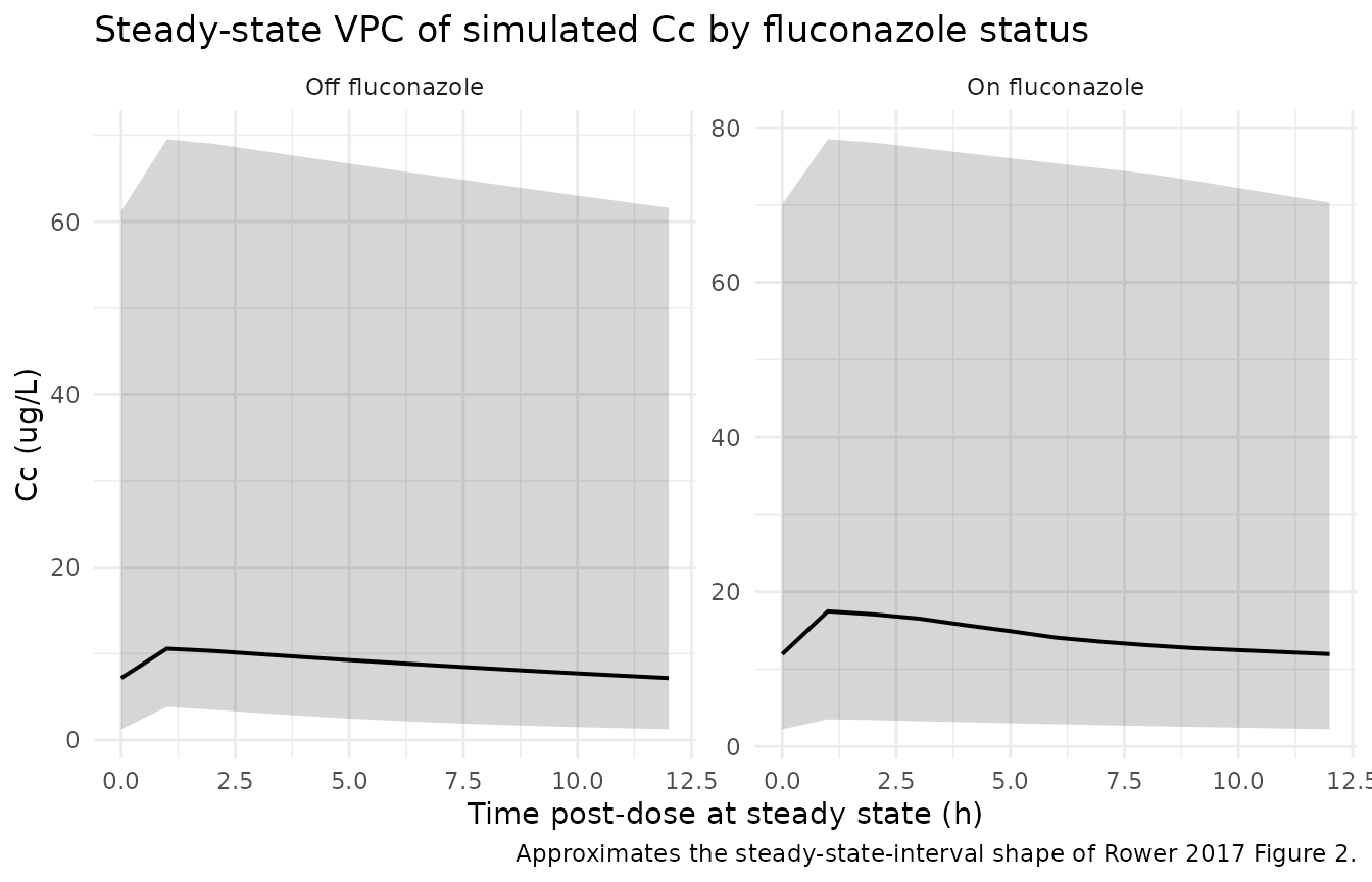

Typical-value profile across age strata

A second view: for a typical (no-IIV) patient on the cohort-typical dose, fix CRCL at the median (122.4 mL/min/1.73 m^2) and walk AGE across infant (1 year), school-age (6 years), and adolescent (15 years) strata to show how the AGE exponent on V/F (and hence on CL/F) propagates through the steady-state profile. Smaller (younger) patients have smaller V/F (and proportionally smaller CL/F), so the typical peak is lower for younger patients on the same 1 mg q12h dose. This is the AGE-on-V/F structural effect of the source model.

age_strata <- tibble(
  id        = 1:3,
  AGE       = c(1, 6, 15),
  CRCL      = 122.4,
  CONMED_AZOLE = 0L,
  treatment = paste0("Age ", c(1, 6, 15), " years")
)

events_age <- build_events(age_strata)
stopifnot(!anyDuplicated(unique(events_age[, c("id", "time", "evid")])))

sim_age <- rxode2::rxSolve(
  mod_typical, events = events_age,
  keep = c("treatment", "AGE", "CRCL"),
  addDosing = FALSE
) |>
  as.data.frame()
#> ℹ omega/sigma items treated as zero: 'etalcl', 'etalvc'
#> Warning: multi-subject simulation without without 'omega'

sim_age |>
  filter(time >= 288, time <= 300) |>
  mutate(time_post_dose = time - 288) |>
  ggplot(aes(time_post_dose, Cc, colour = treatment)) +
  geom_line(linewidth = 0.7) +
  labs(x = "Time post-dose at steady state (h)", y = "Cc (ug/L)",
       colour = NULL,
       title = "Typical-value steady-state profile by AGE stratum",
       caption = "1 mg q12h, no fluconazole, median CRCL; AGE on V/F propagates to CL/F.") +
  theme_minimal()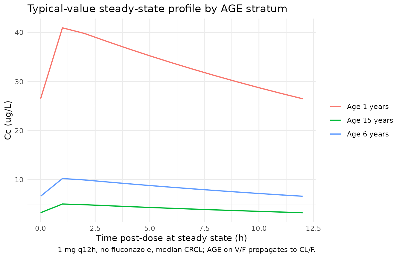

PKNCA validation

Tacrolimus is dosed q12h to steady state in clinical practice. The PKNCA configuration below computes single-dosing-interval Cmax, Tmax, AUClast, and Cmin over the last 12-hour dosing interval at steady state (hours 288 to 300) for each subject and treatment arm.

nca_window_start <- 288
nca_window_end   <- 300

sim_nca <- sim |>
  filter(time >= nca_window_start,
         time <= nca_window_end,
         !is.na(Cc)) |>
  mutate(time_rel = time - nca_window_start) |>
  select(id, time_rel, Cc, treatment)

dose_df <- events |>
  filter(evid == 1, time == nca_window_start) |>
  mutate(time_rel = 0) |>
  select(id, time_rel, amt, treatment)

conc_obj <- PKNCA::PKNCAconc(sim_nca, Cc ~ time_rel | treatment + id,
                             concu = "ug/L",
                             timeu = "h")
dose_obj <- PKNCA::PKNCAdose(dose_df, amt ~ time_rel | treatment + id,
                             doseu = "mg")

intervals <- data.frame(
  start    = 0,
  end      = nca_window_end - nca_window_start,
  cmax     = TRUE,
  tmax     = TRUE,
  auclast  = TRUE,
  cmin     = TRUE
)

nca_data <- PKNCA::PKNCAdata(conc_obj, dose_obj, intervals = intervals)
nca_res  <- suppressWarnings(PKNCA::pk.nca(nca_data))

summary(nca_res)
#>  Interval Start Interval End       treatment  N AUClast (h*ug/L) Cmax (ug/L)
#>               0           12 Off fluconazole 30        115 [153]  12.5 [128]
#>               0           12  On fluconazole 30        179 [143]  17.7 [124]
#>  Cmin (ug/L)          Tmax (h)
#>   6.98 [203] 1.00 [1.00, 1.00]
#>   12.1 [175] 1.00 [1.00, 1.00]
#> 
#> Caption: AUClast, Cmax, Cmin: geometric mean and geometric coefficient of variation; Tmax: median and range; N: number of subjects

Comparison against published parameter estimates

Rower 2017 does not report cohort-aggregated NCA values (Cmax, AUC), but does report the implied population-typical half-life. For a median-covariate non-fluconazole patient, the source parameters give t1/2 = ln(2) / ke = ln(2) / 0.0408 = 17.0 h, within the literature range of 6.8 to 25.6 h cited in the source paper’s Discussion. Under concomitant fluconazole, the implied half-life lengthens to ln(2) / 0.0268 = 25.9 h, consistent with the reported 34% reduction in elimination.

The table below summarises typical-value steady-state troughs (Cmin) for the same regimen across the two arms, showing the higher trough under fluconazole coadministration.

sim_typical |>
  filter(time == 300) |>
  group_by(treatment) |>
  summarise(
    typical_trough_ug_L  = round(mean(Cc), 2),
    implied_halflife_h   = ifelse(CONMED_AZOLE[1] == 1L,
                                  round(log(2) / 0.0268, 1),
                                  round(log(2) / 0.0408, 1)),
    .groups = "drop"
  ) |>
  knitr::kable(caption = "Typical-value steady-state trough per arm (1 mg q12h).")

Typical-value steady-state trough per arm (1 mg q12h).
treatment	typical_trough_ug_L	implied_halflife_h
Off fluconazole	10.58	17.0
On fluconazole	19.24	25.9

# Cross-check: implied half-life from the model's typical CL/F and V/F
# at median-covariate, no-fluconazole conditions should equal
# ln(2) / 0.0408 = 17.0 h to within rounding.
cl_typ <- 0.0408 * 233
v_typ  <- 233
ke_typ <- cl_typ / v_typ
t_half <- log(2) / ke_typ
stopifnot(abs(t_half - 17.0) < 0.1)
cat(sprintf("Typical t1/2 (no fluconazole, median age, median CRCL): %.2f h\n", t_half))
#> Typical t1/2 (no fluconazole, median age, median CRCL): 16.99 h

No tuning was performed; the parameter values come from Rower 2017 Table 2’s final-model column verbatim.

Assumptions and deviations

(ke, V) -> (CL/F, V/F) reparameterisation. The source paper uses NONMEM ADVAN2 TRANS1 with primary thetas on ke and V. The packaged model carries the canonical (CL/F, V/F) decomposition (CL/F = ke V = 9.5064 L/h at reference covariates, V/F = 233 L). All typical concentrations are numerically identical to the source. AGE therefore appears with the same exponent on CL/F and V/F (rather than only on V), because in the (CL/F, V/F) form the V/F dependence on AGE propagates equally to CL/F via CL/F = ke V.
IIV block correlation. The source paper reports diagonal omegas on log(ke) (variance 0.262) and log(V) (variance 0.329); converting to log(CL/F) and log(V/F) under the assumption that eta_ke and eta_V are independent yields the block correlation c(0.591, 0.329, 0.329) (Var(etalcl) = 0.262 + 0.329 = 0.591; Var(etalvc) = 0.329; Cov(etalcl, etalvc) = Var(eta_V) = 0.329). Per-subject ke and V realisations are preserved exactly; only the parameter surface changes.
Demographic distributions. Rower 2017 Table 1 reports medians and ranges only. AGE and CRCL were sampled from truncated lognormals (sd_log = 0.7) with the reported median as the geometric centre and the reported range as truncation bounds. Sex, race, and weight are not used by the final model and so were not generated for the simulation; race and sex distributions are recorded in population metadata for reference.
CONMED_AZOLE labelling. The source paper’s covariate is fluconazole-specific (FLUC). The canonical register entry CONMED_AZOLE (concomitant azole antifungal therapy) generalises across azole antifungals; in this model, the effect should be interpreted as fluconazole-specific because all subjects on azole in the source cohort were on fluconazole.
Dose choice. The simulation arms use 1 mg q12h as a representative mid-cohort dose so any concentration difference can be attributed to the covariate effects rather than to dose. The source cohort used individualised doses driven by trough monitoring (median 0.09 mg/kg/day; range 0.02 to 0.49) – not a fixed regimen.
Bioavailability. F is not estimated in the source model (no F1 on $THETA) and defaults to 1 in the implementation. Almost all tacrolimus concentrations in the source were trough draws, which cannot identify F separately from CL/F.
Postoperative day on ke. During forward selection the source paper found postoperative day to be significantly associated with ke (E_max / EC50 form, with and without a Hill coefficient) but “the inclusion of this covariate caused significant model instability and prevented proper model convergence” and was removed from the final model (Rower 2017 “Population PK model” paragraph 3). The packaged model does not include a postoperative-day effect.
CYP3A5 genotype. Not available in the source cohort (Rower 2017 “Discussion” closing paragraph; retrospective cohort) and not part of the final model. Donor-organ CYP3A5 expression is hypothesised to modulate the fluconazole / tacrolimus interaction in paediatric liver transplant recipients (Discussion, ref. 12); the current model does not encode this stratification because heart transplant recipients keep their native liver and the relevant donor CYP3A5 effect is small and not analysable in the source dataset.