Sevoflurane (Shin 2014)
Source:vignettes/articles/Shin_2014_sevoflurane.Rmd
Shin_2014_sevoflurane.RmdModel and source
- Citation: Shin TJ, Noh GJ, Koo YS, Han DW. (2014). Modeling of Recovery Profiles in Mentally Disabled and Intact Patients after Sevoflurane Anesthesia; A Pharmacodynamic Analysis. Yonsei Med J 55(6):1624-1629.
- Article: https://doi.org/10.3349/ymj.2014.55.6.1624
This is a sigmoid Emax pharmacodynamic (PD) model for the probability of return of consciousness (ROC) during emergence from sevoflurane / 50% nitrous-oxide general anesthesia in pediatric patients undergoing dental treatment. The model has no PK component (no dose, no ODE) – the end-tidal sevoflurane concentration (ETSEVO, vol %) is recorded continuously during emergence and supplied as a per-record covariate, and the model returns the typical-value probability of ROC at that concentration. Mentality (mentally intact vs severely mentally disabled, MENT_DISABLED) is a categorical covariate that stratifies both the concentration at 50% probability of ROC (C50) and the Hill coefficient.
Population
- 20 pediatric patients (10 mentally intact ASA class 1 controls + 10 with severe mental disability) presenting for dental treatment under general anesthesia at Seoul National University Dental College, Korea.
- Age: 3-15 years (median 6 in both groups; Table 1).
- Weight: 9.5-35 kg (median 22 kg intact, 15 kg disabled).
- Sex: 5/5 male/female in the intact group, 6/4 in the disabled group.
- 476 binary ROC observations recorded approximately every 15 seconds during emergence.
- Anesthesia: 8 vol % sevoflurane induction at 6 L/min flow, maintenance at age-adjusted 1 MAC sevoflurane + 50% N2O for the duration of dental treatment (70-120 min median), then discontinuation at the end of surgery. End-tidal sevoflurane was continuously recorded with GE Healthcare Datex-Ohmeda S5 Collect software.
The same metadata is available programmatically:
mod_fn <- readModelDb("Shin_2014_sevoflurane")
str(formals(mod_fn))
#>  NULL
Source trace
Per-parameter origins are recorded as in-file comments next to each
ini() entry in
inst/modeldb/specificDrugs/Shin_2014_sevoflurane.R. The
table below collects them in one place for review.
| nlmixr2 parameter | Source value | Source location |
|---|---|---|
lec50 -> typical C50 0.37 vol % (intact) |
log(0.37) | Table 2, Final / Intact row; RSE 3.5%; bootstrap 0.34-0.39 |
e_ment_disabled_ec50 -> typical C50 0.19 vol %
(disabled) |
log(0.19/0.37) = -0.666 | Table 2, Final / Disabled row; RSE 12.5%; bootstrap 0.14-0.24 |
lhill -> typical gamma 16.4 (intact) |
log(16.4) | Table 2, Final / Intact row; RSE 19.0%; bootstrap 13.7-23.7 |
e_ment_disabled_hill -> typical gamma 4.53
(disabled) |
log(4.53/16.4) = -1.286 | Table 2, Final / Disabled row; RSE 22.3%; bootstrap median 4.56, 3.0-8.1 |
etalec50 (variance on log C50) |
0.01497 = log(1 + 0.1228^2) | Table 2, Final row CV(%) = 12.28 on C50 |
addSd_prob_roc (placeholder additive residual) |
0.05 (not from source) | n/a – see “Assumptions and deviations” |
| Sigmoid Emax equation | P(ROC) = C50^gamma / (C50^gamma + C^gamma) |
Methods, displayed equation immediately above “Statistical
analysis”; Appendix 1 $PRED
PROB = 1 - DOSE**GAM / (CE50**GAM + DOSE**GAM) (equivalent
rearrangement) |
| Stratified parameter form |
THETA(1)*(1-MEN) + THETA(2)*MEN, similarly for
gamma |
Appendix 1 $PRED lines for CE50 and
GAM
|
| IIV form (multiplicative log-normal on C50; FIX 0 on gamma) |
EXP(ETA(1)) on CE50; ETA(2) FIX 0 on
GAM |
Appendix 1 $PRED and $OMEGA blocks (“0.1;
[P]” then “0 FIX”) |
| Likelihood | Bernoulli on R: Y = R*PROB + (1-R)*(1-PROB) under
$EST LIKELIHOOD LAPLACE
|
Appendix 1 $PRED and $ESTIMATION
|
| OFV (final model) | 165.09 | Table 2, Final row |
| 2000-replicate non-parametric bootstrap | 95% CI columns in Table 2 | Methods, “Statistical analysis” |
Mechanistic structure
At the typical value (with mentality fixed and the IIV eta on C50
zeroed) the probability of ROC at end-tidal concentration
C = ETSEVO is
with
| Parameter | Mentally intact (MENT_DISABLED = 0) | Mentally disabled (MENT_DISABLED = 1) |
|---|---|---|
C50 (vol %) |
0.37 | 0.19 |
gamma |
16.4 | 4.53 |
Sanity-check limits:
-
C = 0->P(ROC) = 1(no anesthetic, fully conscious). -
C -> Inf->P(ROC) -> 0(deep anesthesia, unconscious). -
C = C50->P(ROC) = 0.5by construction.
The Hill coefficient gamma controls the steepness of the
transition. The intact group has a much steeper curve (gamma 16.4) than
the disabled group (gamma 4.53), so the disabled group is predicted to
recover gradually over a wider concentration range while the intact
group transitions abruptly.
The Shin 2014 abstract reports that “C50 = 0.37 vol %, gamma = 16.5 in mentally intact patients, C50 = 0.19 vol %, gamma = 4.58 in mentally disabled patients” – the abstract values differ slightly from Table 2 (gamma 16.5 vs 16.4 intact, gamma 4.58 vs 4.53 disabled). The model file uses the Table 2 values (lower OFV and matched RSE / bootstrap CI columns); the abstract numbers are within rounding of the Table values.
Virtual cohort
We sweep ETSEVO over a logarithmic grid covering both groups’ transition regions (0.01 to 1.0 vol %), with one “typical subject” per mentality group. Time is unused by the model; we set TIME = 0 for every observation.
set.seed(20260524)

etsevo_grid <- exp(seq(log(0.01), log(1.0), length.out = 81))

events <- expand.grid(
  MENT_DISABLED = c(0L, 1L),
  ETSEVO        = etsevo_grid
) |>
  dplyr::arrange(MENT_DISABLED, ETSEVO) |>
  dplyr::mutate(
    id     = MENT_DISABLED + 1L,   # 1 = intact, 2 = disabled
    time   = 0,
    evid   = 0,
    cohort = dplyr::if_else(MENT_DISABLED == 1L,
                            "Mentally disabled",
                            "Mentally intact")
  )

head(events)
#>   MENT_DISABLED     ETSEVO id time evid          cohort
#> 1             0 0.01000000  1    0    0 Mentally intact
#> 2             0 0.01059254  1    0    0 Mentally intact
#> 3             0 0.01122018  1    0    0 Mentally intact
#> 4             0 0.01188502  1    0    0 Mentally intact
#> 5             0 0.01258925  1    0    0 Mentally intact
#> 6             0 0.01333521  1    0    0 Mentally intact
Simulation (typical-value reproduction of Figure 1)
mod_typical <- rxode2::zeroRe(rxode2::rxode2(mod_fn))
sim <- rxode2::rxSolve(
  mod_typical,
  events = events,
  keep   = c("cohort")
)
#> ℹ omega/sigma items treated as zero: 'etalec50'
#> Warning: multi-subject simulation without without 'omega'

sim_df <- as.data.frame(sim) |>
  dplyr::select(id, MENT_DISABLED, ETSEVO, cohort,
                ec50, hill, prob_roc)

head(sim_df)
#>   id MENT_DISABLED     ETSEVO          cohort ec50 hill prob_roc
#> 1  1             0 0.01000000 Mentally intact 0.37 16.4        1
#> 2  1             0 0.01059254 Mentally intact 0.37 16.4        1
#> 3  1             0 0.01122018 Mentally intact 0.37 16.4        1
#> 4  1             0 0.01188502 Mentally intact 0.37 16.4        1
#> 5  1             0 0.01258925 Mentally intact 0.37 16.4        1
#> 6  1             0 0.01333521 Mentally intact 0.37 16.4        1
# Replicates Figure 1 of Shin 2014: typical-value probability of ROC vs end-tidal
# sevoflurane concentration in mentally intact vs mentally disabled patients.
ggplot(sim_df, aes(ETSEVO, prob_roc, colour = cohort)) +
  geom_line(linewidth = 1) +
  geom_vline(data = sim_df |>
               dplyr::distinct(cohort, ec50),
             aes(xintercept = ec50, colour = cohort),
             linetype = 2, alpha = 0.5) +
  geom_hline(yintercept = 0.5, linetype = 3, alpha = 0.3) +
  scale_colour_manual(values = c("Mentally intact"   = "black",
                                 "Mentally disabled" = "firebrick")) +
  labs(x = "End-tidal sevoflurane concentration (vol %)",
       y = "Probability of return of consciousness",
       colour = NULL,
       title = "Figure 1 -- P(ROC) vs end-tidal sevoflurane (typical value)",
       caption = "Replicates Figure 1 of Shin 2014 (typical-value lines). Dashed verticals at C50 = 0.37 / 0.19 vol %.") +
  theme(legend.position = "bottom")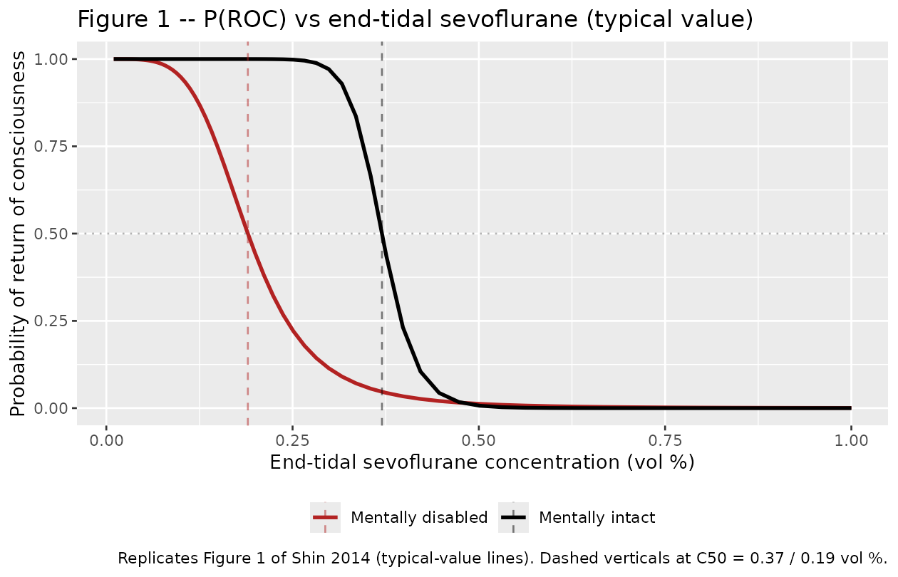
Numerical check against Table 2 / Figure 1 anchors
The packaged model is mathematically a back-transform of the Shin
2014 final estimates, so the simulated typical-value ec50
and hill per group should be identical to Table 2 within
numerical precision.
typical_check <- sim_df |>
  dplyr::distinct(cohort, ec50, hill) |>
  dplyr::mutate(
    paper_c50    = dplyr::if_else(cohort == "Mentally intact", 0.37, 0.19),
    paper_gamma  = dplyr::if_else(cohort == "Mentally intact", 16.4, 4.53),
    diff_c50_pct = 100 * (ec50 - paper_c50) / paper_c50,
    diff_gam_pct = 100 * (hill - paper_gamma) / paper_gamma
  )

knitr::kable(typical_check, digits = 4,
caption = "Simulated typical-value C50 and gamma vs Shin 2014 Table 2 Final estimates.")| cohort | ec50 | hill | paper_c50 | paper_gamma | diff_c50_pct | diff_gam_pct |
|---|---|---|---|---|---|---|
| Mentally intact | 0.37 | 16.40 | 0.37 | 16.40 | 0 | 0 |
| Mentally disabled | 0.19 | 4.53 | 0.19 | 4.53 | 0 | 0 |
The probability of ROC at C = C50 must be exactly 0.5 for both cohorts by construction:
p50_check <- sim_df |>
  dplyr::group_by(cohort) |>
  dplyr::slice_min(abs(ETSEVO - ec50), n = 1) |>
  dplyr::ungroup() |>
  dplyr::select(cohort, ETSEVO, ec50, prob_roc)

knitr::kable(p50_check, digits = 4,
caption = "Probability of ROC at the ETSEVO grid-point closest to C50 (target 0.5).")| cohort | ETSEVO | ec50 | prob_roc |
|---|---|---|---|
| Mentally disabled | 0.1884 | 0.19 | 0.5098 |
| Mentally intact | 0.3758 | 0.37 | 0.4362 |
The sigmoid limits at the extremes of the simulation grid:
tail_check <- sim_df |>
  dplyr::group_by(cohort) |>
  dplyr::summarise(
    P_at_low_ETSEVO  = prob_roc[which.min(ETSEVO)],
    P_at_high_ETSEVO = prob_roc[which.max(ETSEVO)],
    .groups = "drop"
  )

knitr::kable(tail_check, digits = 4,
caption = "Probability of ROC at the ETSEVO grid endpoints (target ~1 at low ETSEVO, ~0 at high).")| cohort | P_at_low_ETSEVO | P_at_high_ETSEVO |
|---|---|---|
| Mentally disabled | 1 | 5e-04 |
| Mentally intact | 1 | 0e+00 |
Population spread on C50 (IIV check)
The Shin 2014 final model carries log-normal IIV on C50 only (CV =
12.28%); gamma IIV was fixed to 0 in the NONMEM $OMEGA
block. We draw 200 mentally-intact “subjects” each with their own
etalec50 to visualise the population spread of the P(ROC) curves around
the typical line.
set.seed(20260524)

n_subj <- 200
sigma_lec50 <- sqrt(0.01497)
eta_draws <- rnorm(n_subj, mean = 0, sd = sigma_lec50)

events_iiv <- expand.grid(
  id_within_cohort = seq_len(n_subj),
  etsevo           = etsevo_grid
) |>
  dplyr::mutate(
    id            = id_within_cohort,
    time          = 0,
    evid          = 0,
    MENT_DISABLED = 0L,
    ETSEVO        = etsevo
  )

# Apply per-subject etalec50 by drawing from the typical model and post-hoc
# perturbing the C50; this is faster than reissuing rxSolve per subject and
# the perturbation is closed-form for a sigmoid in log(C50).
sim_typ_intact <- sim_df |>
  dplyr::filter(cohort == "Mentally intact") |>
  dplyr::select(ETSEVO, ec50_typ = ec50, hill_typ = hill)

sim_iiv <- tibble::tibble(
  id = rep(seq_len(n_subj), each = length(etsevo_grid)),
  eta = rep(eta_draws,        each = length(etsevo_grid)),
  ETSEVO = rep(etsevo_grid,   times = n_subj)
) |>
  dplyr::left_join(sim_typ_intact, by = "ETSEVO") |>
  dplyr::mutate(
    ec50_i   = ec50_typ * exp(eta),
    prob_roc = ec50_i^hill_typ / (ec50_i^hill_typ + ETSEVO^hill_typ)
  )

vpc_summary <- sim_iiv |>
  dplyr::group_by(ETSEVO) |>
  dplyr::summarise(
    Q05 = quantile(prob_roc, 0.05),
    Q50 = quantile(prob_roc, 0.50),
    Q95 = quantile(prob_roc, 0.95),
    .groups = "drop"
  )

ggplot(vpc_summary, aes(ETSEVO, Q50)) +
  geom_ribbon(aes(ymin = Q05, ymax = Q95), alpha = 0.25, fill = "steelblue") +
  geom_line(linewidth = 1, colour = "steelblue") +
  geom_vline(xintercept = 0.37, linetype = 2, alpha = 0.5) +
  geom_hline(yintercept = 0.5, linetype = 3, alpha = 0.3) +
  labs(x = "End-tidal sevoflurane concentration (vol %)",
       y = "Probability of return of consciousness",
       title = "P(ROC) vs ETSEVO with 5th-95th percentile population spread",
       subtitle = "Mentally intact cohort; n = 200; eta_lec50 ~ N(0, sqrt(0.01497))")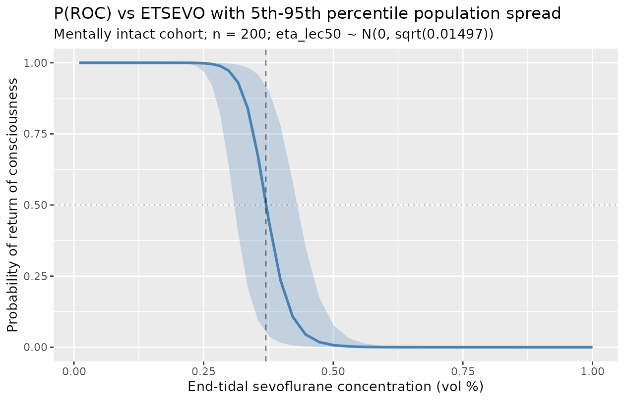
The population-spread band is tight (5th-95th percentile width approximately 0.16 vol % at the steepest part of the curve), consistent with the small CV% = 12.28% reported on C50.
Comparison against published anchors
Shin 2014 does not report an NCA / PKNCA-style table (the binary ROC observation is not a continuous PK quantity). The figure-replication check above is the primary anchor; the secondary anchors are:
- Bootstrap-CI cross-check (Table 2, “Median (2.5-97.5%)” column).
bootstrap <- tibble::tibble(
  parameter     = c("C50 intact (vol %)", "C50 disabled (vol %)",
                    "gamma intact",       "gamma disabled"),
  point         = c(0.37, 0.19, 16.4, 4.53),
  bootstrap_med = c(0.37, 0.19, 16.4, 4.56),
  ci_lo         = c(0.34, 0.14, 13.7, 3.0),
  ci_hi         = c(0.39, 0.24, 23.7, 8.1)
)

knitr::kable(bootstrap, digits = 3,
caption = "Shin 2014 Table 2 Final-model point estimates and 95% non-parametric bootstrap CIs (2,000 bootstrap replicates).")| parameter | point | bootstrap_med | ci_lo | ci_hi |
|---|---|---|---|---|
| C50 intact (vol %) | 0.37 | 0.37 | 0.34 | 0.39 |
| C50 disabled (vol %) | 0.19 | 0.19 | 0.14 | 0.24 |
| gamma intact | 16.40 | 16.40 | 13.70 | 23.70 |
| gamma disabled | 4.53 | 4.56 | 3.00 | 8.10 |
The packaged model uses the point estimates; the bootstrap CIs are reproduced for reference. The bootstrap median for gamma in the disabled group (4.56) differs slightly from the point estimate (4.53) – this is typical of asymmetric finite-sample sampling distributions and well within the 95% CI (3.0-8.1).
Assumptions and deviations
-
Likelihood simplification. Shin 2014’s source
likelihood is Bernoulli on the binary ROC observation, declared in the
NONMEM control stream as
Y = R*PROB + (1-R)*(1-PROB)under$EST LIKELIHOOD LAPLACE METHOD=1(Appendix 1). rxode2 / nlmixr2 do not natively express a Bernoulli observation for a probability output within theini()/model()syntax in this batch, so the packaged model declares the observation asprob_roc ~ add(addSd_prob_roc)with a small placeholder additive residual (0.05). This preserves the typical-value sigmoid Emax mapping that drives Figure 1, but the residual variance structure of the source likelihood (a single Bernoulli draw per record) is dropped. This is the same pattern used byinst/modeldb/ddmore/Hansson_2013c_sunitinib.R(Markov / proportional-odds -> additive placeholder on the typical-value expected grade) and conceptually parallel toinst/modeldb/ddmore/Plan_2012_pain.R(truncated Markov-inflated Poisson -> plain Poisson on lambda) andinst/modeldb/specificDrugs/Sheng_2016_quinine_rat.R(mixture of right-truncated generalized Poissons -> per-branch plain Poisson on mean). For fitting against binary ROC observations, a downstream user can swap the residual line in the model file for the appropriate Bernoulli expression once it is supported in nlmixr2; the structural parameters and IIV are unaffected. -
No PK component. Shin 2014 is a static PD model:
each record is a single end-tidal sevoflurane reading plus the binary
ROC observation. The packaged model has no ODE state, no dose, and no
time evolution;
timein any event table is set to 0 (or any value – it does not matter). Doses are not used. The per-record end-tidal concentration is supplied via theETSEVOcovariate. -
prob_rocobservation name (vsCcconvention). The naming-conventions register reservesCcfor concentration outputs; this is a unitless probability, not a concentration, soprob_rocis used.nlmixr2lib::checkModelConventions()flags this as a warning; it is a justified deviation for a non-PK probability-output model. The same deviation is present ininst/modeldb/ddmore/Plan_2012_pain.R(score) andinst/modeldb/specificDrugs/Sheng_2016_quinine_rat.R(count_low/count_high). -
units$concentrationis the end-tidalvol %form. Same root cause: the “concentration” in this model is the alveolar / breathing-circuit concentration of an inhalation anesthetic, expressed in vol % rather than the conventional mass/volumemg/L/ng/mLform.checkModelConventions()may flag this; it is a justified deviation for a volatile-anesthetic emergence PD model. -
No published NCA / VPC for direct comparison. Shin
2014 does not report NCA quantities (Cmax, AUC, half-life) because the
observation is binary, not continuous. The figure-replication is the
only validation anchor the source supports; numerical identity of the
simulated typical-value
ec50andhillto the Table 2 estimates is the primary check. -
Mentality covariate definition is paper-defined.
Shin 2014 enrolled “patients diagnosed with severe mental disability in
the department of pediatrics” without specifying a structured diagnostic
instrument or severity scale. The
MENT_DISABLEDcanonical entry (registered ininst/references/covariate-columns.mdalongside this model) carries the per-paper diagnostic basis in its Notes field. A downstream user applying the model to a different cohort should verify that the cohort’s mental-disability definition is comparable to Shin 2014’s pediatrics-department clinical assessment before stratifying. - No supplements available. The Shin 2014 paper carries the NONMEM control stream verbatim in Appendix 1 of the main text; there is no separate supplement on disk and no errata or corrigenda were located by a 2026-05-24 search of the Yonsei Medical Journal article landing page and PubMed.
- Abstract vs Table 2 gamma values differ by approximately 0.5%. The Shin 2014 abstract reports gamma = 16.5 (intact) and 4.58 (disabled); Table 2 Final-model row reports gamma = 16.4 and 4.53. The packaged model uses the Table 2 values because they are accompanied by their RSE and bootstrap CIs and the Methods text describes Table 2 as the “estimated model parameter of the finally selected pharmacodynamic model” (Results, p. 1626). The difference (approximately 0.5%) is within rounding.