Model and source
- Citation: Lanke S, Shoaf SE. (2019). Population Pharmacokinetic Analyses and Model Validation of Tolvaptan in Subjects With Autosomal Dominant Polycystic Kidney Disease. J Clin Pharmacol 59(5):763-770. doi:10.1002/jcph.1370
- Description: One-compartment population PK model for oral tolvaptan in adults with autosomal dominant polycystic kidney disease (Lanke 2019): zero-order absorption directly into the central compartment (duration D1), first-order elimination, and a dose-dependent relative bioavailability F1 = Dosemax / (Dose50 + Dose) that falls by about 37 percent from 15 mg to 120 mg per administration. eGFR (power), body weight (power) and CYP3A inhibitor coadministration (fractional change) act on CL/F; body weight (power) acts on Vd/F. Correlated IIV on CL/F, Vd/F and D1, independent IIV on Dose50 and Dosemax, and combined additive plus proportional residual error.
- Article: https://doi.org/10.1002/jcph.1370 (open access, PMC6590359)
Lanke 2019 developed a population PK model of oral tolvaptan, the vasopressin V2-receptor antagonist approved to slow kidney function decline in autosomal dominant polycystic kidney disease (ADPKD), and validated it externally against a separate phase 3b trial. The structural model is one compartment with zero-order absorption (duration D1) directly into the central compartment and first-order elimination. The distinguishing feature is a relative bioavailability that falls with the amount administered,
(Lanke 2019 Equation 4), which the authors attribute to the low solubility of tolvaptan. eGFR, body weight and CYP3A inhibitor coadministration act on CL/F, and body weight acts on Vd/F.
Population
The model was developed from 7335 plasma concentrations in 1091 adults with ADPKD pooled from five phase 2 trials and the phase 3b open-label extension NCT01214421 (Lanke 2019 Methods). Median age was 42 years (range 18-62), median weight 79.5 kg (42.3-164.5), median BMI 25.9 kg/m^2 and median CKD-EPI eGFR 69.4 mL/min/1.73 m^2 (13.62-137.37) (Table 1); 565 of the 1091 subjects were female and 18 were enrolled in Japan (Table 2). Of the 1073 subjects enrolled outside Japan, 1024 were White, 14 Black, 9 Asian, 1 Hispanic and 25 other. Doses ranged from single 15-120 mg doses to split-dose regimens of 15/15 to 90/30 mg, the morning dose at about 8 AM and the second dose 8-9 h later. 131 subjects had at least one record of CYP3A inhibitor coadministration (3.46 percent of observations). External validation used 678 subjects and 3012 observations from the randomized withdrawal trial NCT02160145 at 60/30 or 90/30 mg.
The same information is available programmatically via
readModelDb("Lanke_2019_tolvaptan")$population.
Source trace
| Element | Value | Source location |
|---|---|---|
| Structure: one compartment, zero-order input into central, first-order elimination | – | Results, Base Model; Equation 5 |
lcl (CL/F) |
12.6 L/h | Table 3, Final Model |
lvc (Vd/F) |
110 L | Table 3, Final Model |
ld1 (D1) |
0.58 h | Table 3, Final Model |
lfdepot_dose50 (Dose50) |
166 mg | Table 3, Final Model; Abstract |
lfdepot_dosemax (Dosemax) |
182 mg | Table 3, Final Model; Abstract |
| F1 = Dosemax / (Dose50 + Dose) | – | Equation 4 |
e_crcl_cl (eGFR power on CL/F) |
0.52 | Table 3; normalised to median 69.4 (Table 1, Equation 2) |
e_wt_cl (WT power on CL/F) |
-0.53 | Table 3; normalised to median 79.5 kg (Table 1, Equation 1) |
e_cyp3a4_inh_cl (Inh on CL/F) |
-0.23 | Table 3; linear form of Equation 3 |
e_wt_vc (WT power on Vd/F) |
0.23 | Table 3; Equation 1 |
etalcl, etalvc, etald1
block |
0.40; -0.25, 0.49; 1.13, -1.51, 5.67 | Table 3, Interindividual variability |
etalfdepot_dose50 |
0.086 | Table 3 |
etalfdepot_dosemax |
0.019 | Table 3 |
addSd |
sqrt(5.3) = 2.30 ng/mL | Table 3, Residual variability (variance) |
propSd |
sqrt(0.18) = 0.424 | Table 3, Residual variability (variance) |
The IIV entries are variances: sqrt(0.49) = 70 percent
and sqrt(5.67) = 238 percent reproduce the Abstract’s IIV
for Vd/F and D1, and sqrt(0.40) = 63 percent is the
Abstract’s 64 percent for CL/F to rounding.
mod <- readModelDb("Lanke_2019_tolvaptan")
ui <- rxode2::rxode2(mod)
#> ℹ parameter labels from comments will be replaced by 'label()'
mod_typ <- rxode2::zeroRe(ui)
Dose-dependent bioavailability
The Abstract states that F1 decreased by 36 percent as the dose rose from 15 mg to 120 mg, and the Results state that F1 equals 1 at the lowest dose of 15 mg. Both follow from the Table 3 values. The function decreases monotonically and has no minimum, so the Table 3 footnote’s description of Dosemax (“the highest dose at which F1 is lowest”) does not describe it; likewise F1 reaches 0.5 at 2 x 182 - 166 = 198 mg rather than at Dose50.
f1 <- function(dose) 182 / (166 + dose)
f1_tab <- data.frame(dose_mg = c(15, 30, 45, 60, 90, 120)) |>
  dplyr::mutate(F1 = f1(dose_mg))
knitr::kable(f1_tab, digits = 3, caption = "Typical relative bioavailability by administered amount.")| dose_mg | F1 |
|---|---|
| 15 | 1.006 |
| 30 | 0.929 |
| 45 | 0.863 |
| 60 | 0.805 |
| 90 | 0.711 |
| 120 | 0.636 |
stopifnot(
  abs(f1(15) - 1) < 0.01,
  # Abstract: 'F1 decreased by 36%' from 15 to 120 mg
  abs((1 - f1(120) / f1(15)) * 100 - 36) < 1
)
data.frame(dose = seq(0, 240, by = 1)) |>
  dplyr::mutate(F1 = f1(dose)) |>
  ggplot(aes(dose, F1)) +
  geom_line() +
  geom_point(data = f1_tab, aes(dose_mg, F1)) +
  labs(x = "Tolvaptan amount per administration (mg)", y = "Relative bioavailability F1") +
  theme_bw()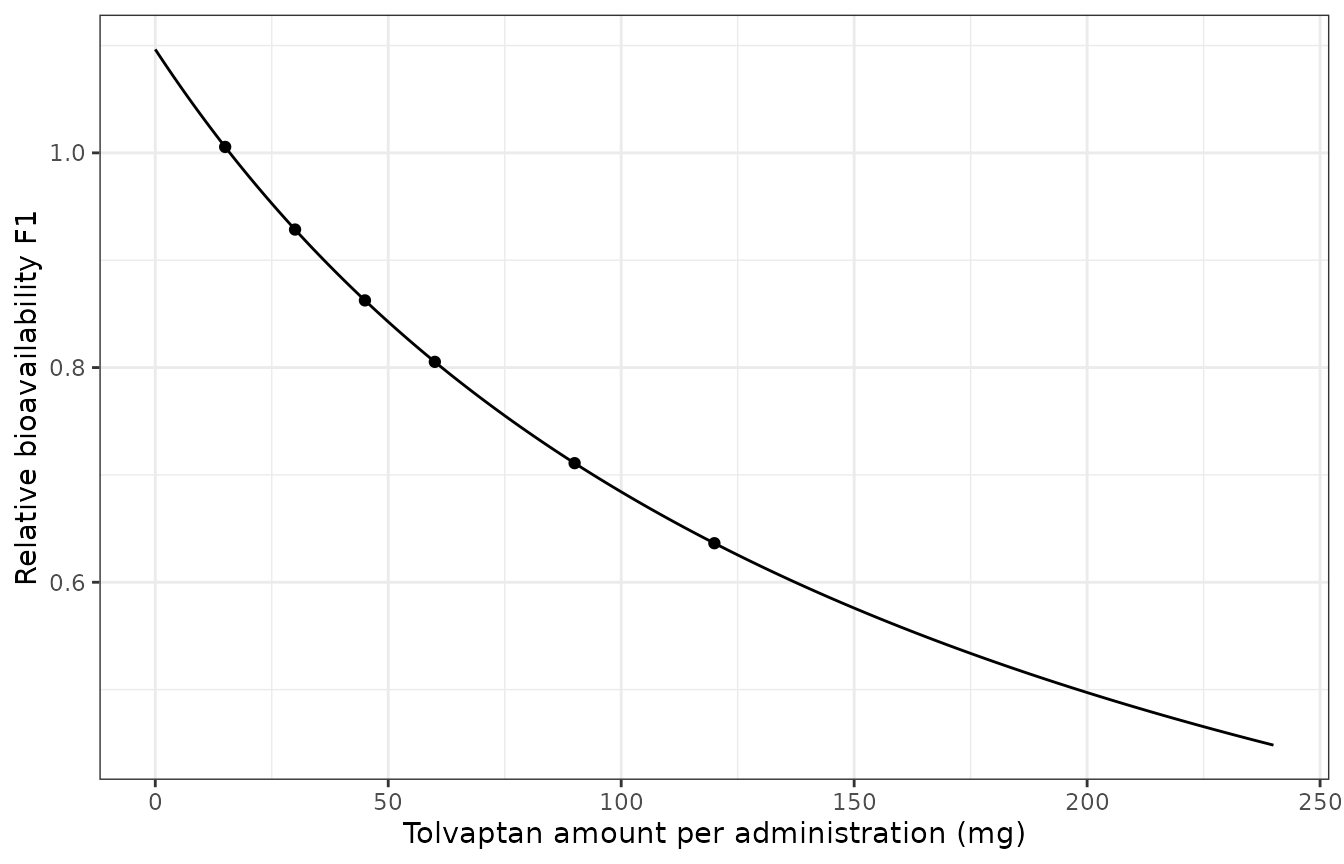
Typical relative bioavailability F1 versus the administered amount (Lanke 2019 Equation 4).
The same ratio must come out of the packaged model. Typical-value
single doses of 15, 30, 60 and 120 mg are simulated in a subject at the
covariate medians, and the PKNCA dose-normalised AUC is compared with
the closed form F1(dose) x dose / CL.
sd_doses <- c(15, 30, 60, 120)
sd_times <- c(seq(0, 2, by = 0.02), seq(2.1, 24, by = 0.1), seq(24.5, 200, by = 0.5))
sd_events <- dplyr::bind_rows(
  data.frame(id = seq_along(sd_doses), time = 0, evid = 1, amt = sd_doses, rate = -2, cmt = "central"),
  tidyr::expand_grid(id = seq_along(sd_doses), time = sd_times) |>
    dplyr::mutate(evid = 0, amt = 0, rate = 0, cmt = "central")
) |>
  dplyr::arrange(id, time, dplyr::desc(evid)) |>
  dplyr::mutate(
    dose_group = paste(sd_doses[id], "mg"),
    DOSE_TOLVAPTAN_MG = sd_doses[id],
    WT = 79.5, CRCL = 69.4, CONMED_CYP3A4_INH = 0
  )

sd_sim <- as.data.frame(rxode2::rxSolve(mod_typ, sd_events, returnType = "data.frame",
                                        keep = "dose_group"))
#> ℹ omega/sigma items treated as zero: 'etalcl', 'etalvc', 'etald1', 'etalfdepot_dose50', 'etalfdepot_dosemax'
#> Warning: multi-subject simulation without without 'omega'

sd_conc <- PKNCA::PKNCAconc(
  dplyr::filter(sd_sim, !is.na(Cc)) |> dplyr::select(id, time, Cc, dose_group),
  Cc ~ time | dose_group + id, concu = "ng/mL", timeu = "h"
)
sd_dose <- PKNCA::PKNCAdose(
  dplyr::filter(sd_events, evid == 1) |> dplyr::select(id, time, amt, dose_group),
  amt ~ time | dose_group + id, doseu = "mg"
)
sd_res <- PKNCA::pk.nca(PKNCA::PKNCAdata(
  sd_conc, sd_dose,
  intervals = data.frame(start = 0, end = Inf, cmax = TRUE, tmax = TRUE,
                         aucinf.obs = TRUE, half.life = TRUE)
))
sd_auc <- as.data.frame(sd_res) |>
  dplyr::filter(PPTESTCD == "aucinf.obs") |>
  dplyr::mutate(
    dose = sd_doses[id],
    closed_form = 1000 * f1(dose) * dose / 12.6,
    pct_diff = 100 * (PPORRES - closed_form) / closed_form,
    auc_per_mg = PPORRES / dose
  )
knitr::kable(
  sd_auc |>
    dplyr::select(dose_group, PPORRES, closed_form, pct_diff, auc_per_mg) |>
    dplyr::rename(
      "Dose" = dose_group, "AUC0-inf simulated (ng*h/mL)" = PPORRES,
      "AUC0-inf closed form (ng*h/mL)" = closed_form,
      "Difference (percent)" = pct_diff, "AUC per mg" = auc_per_mg
    ),
  digits = 2, caption = "Typical-value single-dose AUC0-inf from PKNCA against F1 x Dose / CL."
)| Dose | AUC0-inf simulated (ng*h/mL) | AUC0-inf closed form (ng*h/mL) | Difference (percent) | AUC per mg |
|---|---|---|---|---|
| 120 mg | 6060.60 | 6060.61 | 0 | 50.51 |
| 15 mg | 1197.05 | 1197.05 | 0 | 79.80 |
| 30 mg | 2210.88 | 2210.88 | 0 | 73.70 |
| 60 mg | 3834.81 | 3834.81 | 0 | 63.91 |
# Same parameters on both sides, so only quadrature error separates them.
stopifnot(all(abs(sd_auc$pct_diff) < 1))
auc_ratio <- with(sd_auc, auc_per_mg[dose == 120] / auc_per_mg[dose == 15])
stopifnot(abs((1 - auc_ratio) * 100 - 36) < 1.5)
The dose-normalised AUC at 120 mg is 63.3 percent of that at 15 mg, the 36 percent decrease the Abstract reports.
Covariate effects (replicates Figure 1)
The Results give the covariate effects at the 5th and 95th percentiles of eGFR (32 and 110 mL/min/1.73 m^2) and body weight (56 and 113 kg) relative to the median subject; the Discussion gives the effect of inhibitor coadministration. These are the bars of Lanke 2019 Figure 1.
The typical CL/F and Vd/F are read from a typical-value solve of the
packaged model for each covariate scenario, so the check exercises the
model() equations rather than a re-typed formula.
scen <- tibble::tribble(
  ~scenario, ~WT, ~CRCL, ~CONMED_CYP3A4_INH,
  "median", 79.5, 69.4, 0,
  "eGFR 32", 79.5, 32, 0,
  "eGFR 110", 79.5, 110, 0,
  "WT 56 kg", 56, 69.4, 0,
  "WT 113 kg", 113, 69.4, 0,
  "CYP3A inhibitor", 79.5, 69.4, 1
) |>
  dplyr::mutate(id = dplyr::row_number())
scen_events <- dplyr::bind_rows(
  dplyr::mutate(scen, time = 0, evid = 1, amt = 15, rate = -2),
  dplyr::mutate(scen, time = 1, evid = 0, amt = 0, rate = 0)
) |>
  dplyr::mutate(cmt = "central", DOSE_TOLVAPTAN_MG = 15) |>
  dplyr::select(id, time, evid, amt, rate, cmt, DOSE_TOLVAPTAN_MG, WT, CRCL, CONMED_CYP3A4_INH, scenario) |>
  dplyr::arrange(id, time)
scen_par <- as.data.frame(rxode2::rxSolve(mod_typ, scen_events, returnType = "data.frame",
                                          keep = "scenario")) |>
  dplyr::distinct(scenario, cl, vc)
#> ℹ omega/sigma items treated as zero: 'etalcl', 'etalvc', 'etald1', 'etalfdepot_dose50', 'etalfdepot_dosemax'
#> Warning: multi-subject simulation without without 'omega'
ref <- dplyr::filter(scen_par, scenario == "median")
stopifnot(abs(ref$cl - 12.6) < 1e-6, abs(ref$vc - 110) < 1e-6)

cov_tab <- tibble::tribble(
  ~parameter, ~covariate, ~published_pct,
  "CL/F", "eGFR 32", -33,
  "CL/F", "eGFR 110", 27,
  "CL/F", "WT 56 kg", 20,
  "CL/F", "WT 113 kg", -17,
  "CL/F", "CYP3A inhibitor", -23,
  "Vd/F", "WT 56 kg", -8,
  "Vd/F", "WT 113 kg", 8
) |>
  dplyr::left_join(scen_par, by = c("covariate" = "scenario")) |>
  dplyr::mutate(
    value = ifelse(parameter == "CL/F", cl / ref$cl, vc / ref$vc),
    model_pct = 100 * (value - 1)
  )

knitr::kable(
  cov_tab |>
    dplyr::select(parameter, covariate, model_pct, published_pct) |>
    dplyr::rename(
      "Parameter" = parameter, "Covariate value" = covariate,
      "Model change (percent)" = model_pct, "Published change (percent)" = published_pct
    ),
  digits = 1,
  caption = "Covariate effects against the Lanke 2019 Results and Discussion."
)| Parameter | Covariate value | Model change (percent) | Published change (percent) |
|---|---|---|---|
| CL/F | eGFR 32 | -33.1 | -33 |
| CL/F | eGFR 110 | 27.1 | 27 |
| CL/F | WT 56 kg | 20.4 | 20 |
| CL/F | WT 113 kg | -17.0 | -17 |
| CL/F | CYP3A inhibitor | -23.0 | -23 |
| Vd/F | WT 56 kg | -7.7 | -8 |
| Vd/F | WT 113 kg | 8.4 | 8 |
cov_tab |>
  dplyr::mutate(label = paste(parameter, covariate)) |>
  ggplot(aes(x = model_pct, y = reorder(label, model_pct))) +
  geom_col(width = 0.6, orientation = "y") +
  geom_vline(xintercept = c(-20, 25), linetype = "dashed") +
  labs(x = "Change from the median subject (percent)", y = NULL) +
  theme_bw()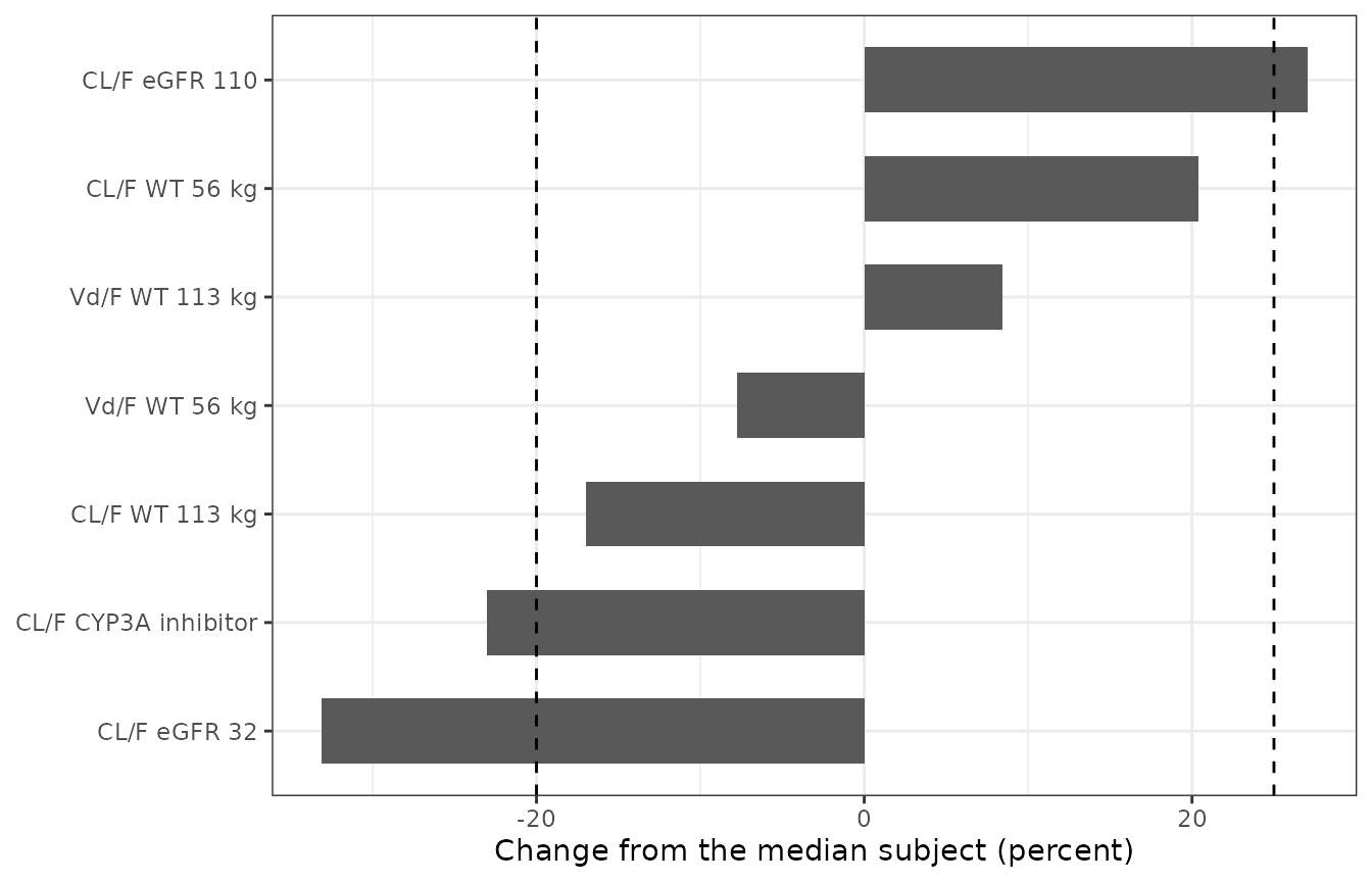
Replicates Figure 1 of Lanke 2019: change in CL/F and Vd/F at the 5th and 95th covariate percentiles. Dashed lines mark 80 and 125 percent.
The Discussion also gives CL/F of 14.7 L/h at 56 kg and 10.2 L/h at 113 kg against “the typical value of 12.3 L/h”. The model gives 15.2 and 10.5 L/h from the Table 3 value of 12.6 L/h; the ratios to the typical value agree to within 1 percent, and only the typical value differs (see Assumptions and deviations).
Virtual cohort
97 percent of the development observations, and 93.7 percent of the validation observations, came from the 60/30 and 90/30 mg split-dose regimens, so the stochastic simulation uses those two arms with 200 subjects each. Body weight is log-normal around the median of 79.5 kg with the dispersion implied by the published 5th and 95th percentiles (56 and 113 kg); eGFR is normal around 69.4 with the dispersion implied by its percentiles (32 and 110), truncated to the observed range. CYP3A inhibitor coadministration is drawn per subject with the 3.46 percent observation-level frequency of Table 2 and held constant within a subject.
rxode2::rxSetSeed(20190501)
n_per_arm <- 200
regimens <- tibble::tribble(
  ~regimen, ~am_mg, ~pm_mg,
  "60/30 mg", 60, 30,
  "90/30 mg", 90, 30
)
cohort <- tidyr::expand_grid(regimen = regimens$regimen, subj = seq_len(n_per_arm)) |>
  dplyr::mutate(
    id = dplyr::row_number(),
    WT = pmin(pmax(79.5 * exp(rnorm(dplyr::n(), 0, log(113 / 56) / (2 * 1.645))), 42.3), 164.5),
    CRCL = pmin(pmax(rnorm(dplyr::n(), 69.4, (110 - 32) / (2 * 1.645)), 13.62), 137.37),
    CONMED_CYP3A4_INH = rbinom(dplyr::n(), 1, 0.0346)
  ) |>
  dplyr::left_join(regimens, by = "regimen")

knitr::kable(
  cohort |>
    dplyr::group_by(regimen) |>
    dplyr::summarise(
      n = dplyr::n(), WT_median = median(WT), CRCL_median = median(CRCL),
      CRCL_p05 = quantile(CRCL, 0.05), CRCL_p95 = quantile(CRCL, 0.95),
      inh_pct = 100 * mean(CONMED_CYP3A4_INH)
    ),
  digits = 1, caption = "Virtual cohort summary."
)| regimen | n | WT_median | CRCL_median | CRCL_p05 | CRCL_p95 | inh_pct |
|---|---|---|---|---|---|---|
| 60/30 mg | 200 | 81.5 | 65.3 | 27.9 | 105.3 | 3 |
| 90/30 mg | 200 | 80.1 | 68.7 | 32.2 | 102.6 | 4 |
Simulation
Fourteen days of split dosing: the morning dose at 0 h of each day
and the afternoon dose 8 h later, both as modelled-duration zero-order
input (rate = -2). DOSE_TOLVAPTAN_MG carries
the amount of each administration, so the morning and afternoon doses
get different bioavailabilities. Day 14 (312-336 h) is sampled
densely.
n_days <- 14
ss_start <- (n_days - 1) * 24
ss_end <- n_days * 24
dose_rows <- cohort |>
  tidyr::expand_grid(day = seq_len(n_days) - 1, slot = c("am", "pm")) |>
  dplyr::mutate(
    time = 24 * day + ifelse(slot == "am", 0, 8),
    amt = ifelse(slot == "am", am_mg, pm_mg),
    evid = 1, rate = -2, cmt = "central"
  )
obs_rows <- cohort |>
  tidyr::expand_grid(time = c(seq(ss_start, ss_start + 2, by = 0.05),
                              seq(ss_start + 2.1, ss_start + 10, by = 0.05),
                              seq(ss_start + 10.1, ss_end, by = 0.1))) |>
  dplyr::mutate(evid = 0, amt = 0, rate = 0, cmt = "central")
events <- dplyr::bind_rows(dose_rows, obs_rows) |>
  dplyr::arrange(id, time, dplyr::desc(evid)) |>
  dplyr::group_by(id) |>
  dplyr::mutate(DOSE_TOLVAPTAN_MG = ifelse(evid == 1, amt, NA_real_)) |>
  tidyr::fill(DOSE_TOLVAPTAN_MG, .direction = "down") |>
  dplyr::ungroup() |>
  dplyr::select(id, time, evid, amt, rate, cmt, DOSE_TOLVAPTAN_MG, WT, CRCL,
                CONMED_CYP3A4_INH, regimen, am_mg, pm_mg)

sim <- as.data.frame(rxode2::rxSolve(
  ui, events, returnType = "data.frame",
  keep = c("regimen", "am_mg", "pm_mg")
))
sim |>
  dplyr::filter(time >= ss_start) |>
  dplyr::mutate(tad_day = time - ss_start) |>
  dplyr::group_by(regimen, tad_day) |>
  dplyr::summarise(
    p05 = quantile(Cc, 0.05), p50 = median(Cc), p95 = quantile(Cc, 0.95),
    .groups = "drop"
  ) |>
  ggplot(aes(tad_day, p50)) +
  geom_ribbon(aes(ymin = p05, ymax = p95), alpha = 0.25) +
  geom_line() +
  facet_wrap(~regimen) +
  scale_y_log10() +
  labs(x = "Time after the day-14 morning dose (h)", y = "Tolvaptan (ng/mL)") +
  theme_bw()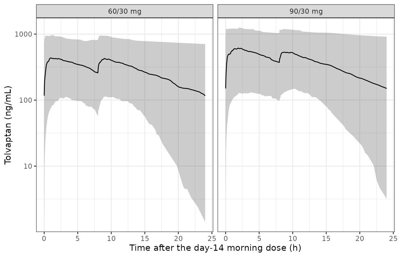
Simulated day-14 tolvaptan concentrations by regimen: median and 5th-95th percentile band of the individual predictions (compare the external-validation VPC of Lanke 2019 Figure 2).
PKNCA validation
Lanke 2019 reports no NCA summary for its simulations, so the
steady-state NCA is checked against the closed form it must satisfy
instead. For any subject at steady state the AUC over one day equals the
bioavailable daily amount divided by clearance,
AUC0-24 = 1000 x (F1(AM) x AM + F1(PM) x PM) / CL, whatever
the absorption duration. Both sides use the same drawn parameters, so
the check fails on a mis-applied bioavailability (for example the daily
total instead of the per-administration amount, or a bioavailability
that is not evaluated on its own dose record).
nca_conc <- sim |>
  dplyr::filter(!is.na(Cc), time >= ss_start) |>
  dplyr::select(id, time, Cc, regimen)
nca_dose <- events |>
  dplyr::filter(evid == 1, time >= ss_start) |>
  dplyr::select(id, time, amt, regimen)

conc_obj <- PKNCA::PKNCAconc(nca_conc, Cc ~ time | regimen + id, concu = "ng/mL", timeu = "h")
dose_obj <- PKNCA::PKNCAdose(nca_dose, amt ~ time | regimen + id, doseu = "mg")
intervals <- data.frame(start = ss_start, end = ss_end, cmax = TRUE, tmax = TRUE,
                        cmin = TRUE, auclast = TRUE)
nca_res <- suppressMessages(PKNCA::pk.nca(PKNCA::PKNCAdata(conc_obj, dose_obj, intervals = intervals)))
knitr::kable(summary(nca_res), caption = "Simulated day-14 NCA per regimen (one dosing day, 24 h).")| Interval Start | Interval End | regimen | N | AUClast (h*ng/mL) | Cmax (ng/mL) | Cmin (ng/mL) | Tmax (h) |
|---|---|---|---|---|---|---|---|
| 312 | 336 | 60/30 mg | 200 | 6510 [92.8] | 446 [79.0] | 76.1 [691] | 2.18 [0.0500, 23.7] |
| 312 | 336 | 90/30 mg | 200 | 8670 [82.5] | 615 [65.4] | 107 [472] | 0.550 [0.0500, 23.1] |
indiv <- sim |>
  dplyr::filter(time == ss_start) |>
  dplyr::distinct(id, regimen, am_mg, pm_mg, cl, fdepot_dose50, fdepot_dosemax, d1)
chk <- as.data.frame(nca_res) |>
  dplyr::filter(PPTESTCD == "auclast") |>
  dplyr::select(id, regimen, auc_sim = PPORRES) |>
  dplyr::left_join(indiv, by = c("id", "regimen")) |>
  dplyr::mutate(
    auc_closed = 1000 * (am_mg * fdepot_dosemax / (fdepot_dose50 + am_mg) +
                           pm_mg * fdepot_dosemax / (fdepot_dose50 + pm_mg)) / cl,
    pct_diff = 100 * (auc_sim - auc_closed) / auc_closed
  )
knitr::kable(
  chk |>
    dplyr::group_by(regimen) |>
    dplyr::summarise(
      median_auc_sim = median(auc_sim), median_auc_closed = median(auc_closed),
      median_pct_diff = median(pct_diff), p90_abs_pct_diff = quantile(abs(pct_diff), 0.9)
    ) |>
    dplyr::rename(
      "Regimen" = regimen, "Median AUC0-24 simulated (ng*h/mL)" = median_auc_sim,
      "Median AUC0-24 closed form (ng*h/mL)" = median_auc_closed,
      "Median difference (percent)" = median_pct_diff,
      "90th percentile absolute difference (percent)" = p90_abs_pct_diff
    ),
  digits = 2, caption = "Steady-state AUC0-24 from PKNCA against the per-subject closed form."
)| Regimen | Median AUC0-24 simulated (ng*h/mL) | Median AUC0-24 closed form (ng*h/mL) | Median difference (percent) | 90th percentile absolute difference (percent) |
|---|---|---|---|---|
| 60/30 mg | 6833.32 | 6833.95 | -0.01 | 0.06 |
| 90/30 mg | 9186.58 | 9186.93 | 0.00 | 0.16 |
# Centre and robust envelope only: subjects with a very long D1 (IIV variance
# 5.67) are still approaching steady state on day 14.
stopifnot(
  abs(median(chk$pct_diff)) < 1,
  quantile(abs(chk$pct_diff), 0.9) < 5
)
A typical subject at the covariate medians is checked the same way with no random effects.
typ_events <- events |>
  dplyr::filter(id %in% c(1, n_per_arm + 1)) |>
  dplyr::mutate(WT = 79.5, CRCL = 69.4, CONMED_CYP3A4_INH = 0)
typ_sim <- as.data.frame(rxode2::rxSolve(mod_typ, typ_events, returnType = "data.frame",
                                         keep = c("regimen", "am_mg", "pm_mg")))
#> ℹ omega/sigma items treated as zero: 'etalcl', 'etalvc', 'etald1', 'etalfdepot_dose50', 'etalfdepot_dosemax'
#> Warning: multi-subject simulation without without 'omega'
typ_chk <- typ_sim |>
  dplyr::filter(time >= ss_start) |>
  dplyr::group_by(regimen, am_mg, pm_mg) |>
  dplyr::summarise(
    auc_sim = sum(diff(time) * (head(Cc, -1) + tail(Cc, -1)) / 2),
    .groups = "drop"
  ) |>
  dplyr::mutate(
    auc_closed = 1000 * (am_mg * f1(am_mg) + pm_mg * f1(pm_mg)) / 12.6,
    pct_diff = 100 * (auc_sim - auc_closed) / auc_closed
  )
knitr::kable(typ_chk, digits = 2, caption = "Typical-subject steady-state AUC0-24.")| regimen | am_mg | pm_mg | auc_sim | auc_closed | pct_diff |
|---|---|---|---|---|---|
| 60/30 mg | 60 | 30 | 6045.37 | 6045.69 | -0.01 |
| 90/30 mg | 90 | 30 | 7288.61 | 7289.01 | -0.01 |
Comparison against published NCA
Lanke 2019 reports no Cmax, AUC or half-life values for tolvaptan, so there is no published NCA table to compare against. The quantitative checks above replace it: the 36 percent fall in F1 from the Abstract, the covariate effects from the Results and Discussion, and the closed-form steady-state exposure.
Assumptions and deviations
- Dose50 = 166 mg, not 160 mg. The Results prose gives Dose50 as 160 mg; Table 3 and the Abstract give 166 mg. 166 mg is used because it makes F1 equal to 1 at 15 mg (182 / 181 = 1.006), as the Results state, and reproduces the Abstract’s 36 percent decrease from 15 to 120 mg (36.7 percent); 160 mg gives 1.04 and 37.5 percent.
-
Residual error read as variances. Table 3 prints
Additive 5.3 and Proportional 0.18 without saying whether they are
variances or standard deviations, and no control stream is published.
They are read as NONMEM SIGMA variances (
addSd = sqrt(5.3)= 2.30 ng/mL,propSd = sqrt(0.18)= 0.424), consistent with the IIV block of the same table, which is provably on the variance scale. This was a maintainer ruling; it affects only the spread of simulated observations, notCc. -
Per-administration dose in F1. Equation 4 does not
say whether
Doseis the amount of each administration or the daily total. The model uses the amount of each administration, carried inDOSE_TOLVAPTAN_MG, because the paper anchors F1 to the lowest single dose of 15 mg, which is also the smallest administration in any split regimen. -
New parameter names.
lfdepot_dose50andlfdepot_dosemaxwere registered for the two dose-scale constants (maintainers’ ruling), following thelcl_dose50grammar of the dose-dependent clearance family. The paper’s own glosses for them (“the dose at which F1 is 50%”, “the highest dose at which F1 is lowest”) do not describe Equation 4. - Typical CL/F in the Discussion. The Discussion computes the body-weight examples (14.7 and 10.2 L/h) from a typical CL/F of 12.3 L/h, whereas Table 3 gives 12.6 L/h. The model uses Table 3; the ratios are the same.
- F1 is relative. Only oral data were modelled, so F1 is relative to a 15 mg administration and CL/F and Vd/F are apparent values.
- Food not modelled. Food intake was not recorded in the phase 3b trials, and the paper notes that a high-fat meal raised Cmax by 15-96 percent; there is no food effect in the model.
- Virtual cohort. Body weight and eGFR distributions are reconstructed from the published medians and 5th/95th percentiles; CYP3A inhibitor use is a per-subject indicator drawn at the observation-level frequency, whereas in the source data it changed record by record. The CYP3A4 inducer indicator, age, BMI, sex and Japan site were screened but are not in the final model.