Ethambutol for Mycobacterium kansasii lung disease (Gumbo 2026)
Source:vignettes/articles/Gumbo_2026_ethambutol.Rmd
Gumbo_2026_ethambutol.RmdModel and source
Gumbo 2026 studied ethambutol against Mycobacterium kansasii complex (MKC) in a hollow fiber system model (HFS-MKC) and then ran Monte Carlo experiments to choose a clinical dose. The paper contributes two models to nlmixr2lib:
Gumbo_2026_ethambutol: the human plasma PK prior of the Monte Carlo experiments, a two-compartment oral model.Gumbo_2026_ethambutol_hfs: the hollow-fiber exposure-response fits. For each sampling day there is an inhibitory sigmoid Emax curve of total burden (log10 CFU/mL and MGIT time-to-positivity) against AUC0-24/MIC (Table 2), plus the U-shaped quadratic of the ethambutol-resistant subpopulation (Figure 4C).Citation: Gumbo T, Boorgula GD, Srivastava S. Preclinical pharmacokinetics/pharmacodynamics studies defining the role of ethambutol in Mycobacterium kansasii lung disease. Antimicrob Agents Chemother. 2026;70(2):e01447-25. doi:10.1128/aac.01447-25. PK parameters from Materials and Methods, ‘Monte Carlo experiments’.
Article: https://doi.org/10.1128/aac.01447-25 (open access, PMC12888887)
mod_pk <- readModelDb("Gumbo_2026_ethambutol")
mod_hfs <- readModelDb("Gumbo_2026_ethambutol_hfs")
Population
Human PK prior. This is not a fitted cohort. Gumbo 2026 put the five PK parameters and their between-subject variability into the ADAPT 5 “subroutine prior” from previously published ethambutol population PK and lung-cavity studies (its references 11, 18 and 19). Clearance is the value for the average 64 kg MKC lung-disease patient in Poland with normal renal function. Weight and renal function were deliberately left out, and protein binding was assumed to be negligible. Monte Carlo experiments simulated 10,000 virtual patients for each of 600, 1,200, 1,800, 2,400 and 3,000 mg once daily.
Hollow fiber system. Eight HFS-MKC units were inoculated with THP-1 monocytes infected with the reference strain ATCC 12478 (ethambutol MIC 8 mg/L): six once-daily ethambutol regimens (R1-R6) and two non-treated controls. The units ran for 21 days. Ethambutol was infused over 1 h, with the dilution rate set to mimic unbound concentrations at the centre of tuberculosis lung cavities. The AUC0-24/MIC exposures of R1-R6 were 0.13, 0.28, 0.5, 1.41, 1.74 and 2.07 (Figure 3 panel titles). Bacterial burden was sampled on days 4, 7, 14 and 21. The day-0 burden (B0) was about 5.3 log10 CFU/mL, and no exposure killed below B0.
Source trace
| Item | Value | Source |
|---|---|---|
| Structure (human PK) | 2-compartment, first-order absorption, linear elimination | Methods, “Monte Carlo experiments” |
lka |
0.498 1/h (IIV 43%) | Methods, “Monte Carlo experiments” |
lcl |
39.7 L/h at 64 kg (IIV 34%) | Methods, “Monte Carlo experiments” |
lvc |
90 L (IIV 40%) | Methods, “Monte Carlo experiments” |
lq |
33.8 L/h (IIV 40%) | Methods, “Monte Carlo experiments” |
lvp |
642 L (IIV 40%) | Methods, “Monte Carlo experiments” |
eta* variances |
log(1 + CV^2) | IIV percentages read as log-normal CV (see Assumptions) |
propSd |
0 (fixed) | not reported |
| Exposure index (HFS) | AUC0-24/MIC = AUC_ETHAMBUTOL / mic
|
Methods, “Data analysis”; Figure 2B and Figure 3 titles |
mic |
8 mg/L (fixed) | Results, first paragraph |
CFU readout: le0_cfu_d*, lemax_cfu_d*,
lhill_cfu_d*, lec50_cfu_d*
|
per day | Table 2, “CFU/mL readout” |
TTP readout: le0_ttp_d*, lemax_ttp_d*,
lhill_ttp_d*, lec50_ttp_d*
|
per day | Table 2, “Time-to-positivity readout” |
| Total burden equation | log_cfu = Econ - Emax X^H / (X^H + EC50^H) | Methods, “Data analysis” (inhibitory sigmoid Emax) |
| TTP equation | ttp = Econ + Emax X^H / (X^H + EC50^H) | Table 2 with Figure 4A (TTP rises with exposure) |
| Resistant equation | log_cfu_res = res0 + res1 X + res2 X^2 | Methods, “Data analysis” (quadratic) |
res0_d*, res1_d*,
res2_d*
|
per day | digitised by the maintainers from Figure 4C |
| Residual SDs (HFS) | 0 (fixed) | Table 2 reports r2 only |
Human PK prior
Virtual cohort and simulation
Each of the five Monte Carlo doses gets 200 virtual patients, which is enough to show the PK and keeps the article quick to build. They are sampled densely over the first 24 h after a single dose.
doses <- c(600, 1200, 1800, 2400, 3000)
n_per_arm <- 200
obs_times <- seq(0, 24, by = 0.5)

pk_events <- bind_rows(lapply(seq_along(doses), function(i) {
  ids <- (i - 1) * n_per_arm + seq_len(n_per_arm)
  dose_rows <- data.frame(id = ids, time = 0, amt = doses[i], evid = 1L, cmt = "depot")
  obs_rows <- expand.grid(id = ids, time = obs_times)
  obs_rows$amt <- 0
  obs_rows$evid <- 0L
  obs_rows$cmt <- "central"
  bind_rows(dose_rows, obs_rows) |> mutate(dose = doses[i])
})) |>
  arrange(id, time, desc(evid))

rxode2::rxSetSeed(20261)
pk_sim <- rxode2::rxSolve(mod_pk, events = pk_events, keep = "dose", returnType = "data.frame")
#> ℹ parameter labels from comments will be replaced by 'label()'
pk_sim |>
  group_by(dose, time) |>
  summarise(
    med = median(Cc), lo = quantile(Cc, 0.05), hi = quantile(Cc, 0.95),
    .groups = "drop"
  ) |>
  mutate(dose = factor(paste(dose, "mg"), levels = paste(doses, "mg"))) |>
  ggplot(aes(time, med, colour = dose, fill = dose)) +
  geom_ribbon(aes(ymin = lo, ymax = hi), alpha = 0.15, colour = NA) +
  geom_line() +
  labs(x = "Time after dose (h)", y = "Plasma ethambutol (mg/L)", colour = NULL, fill = NULL)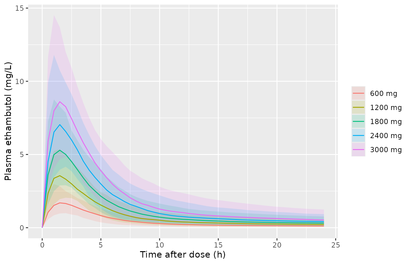
Simulated plasma ethambutol after a single oral dose (median and 90% prediction interval, 200 virtual patients per dose).
Closed-form check
At steady state the dosing-interval AUC of a linear model equals dose / CL, whatever the absorption and distribution. A typical-value solve over 30 days of 1,200 mg once daily has to reproduce 1200 / 39.7 = 30.23 mg*h/L. Because the solve is checked against its own closed form, a tight tolerance is appropriate.
ss_events <- rxode2::et(amt = 1200, cmt = "depot", ii = 24, addl = 29) |>
  rxode2::et(seq(696, 720, by = 0.05), cmt = "central")
ss <- rxode2::rxSolve(rxode2::zeroRe(mod_pk), ss_events, returnType = "data.frame")
#> ℹ parameter labels from comments will be replaced by 'label()'
#> ℹ omega/sigma items treated as zero: 'etalka', 'etalcl', 'etalvc', 'etalq', 'etalvp'
auc_ss <- sum(diff(ss$time) * (head(ss$Cc, -1) + tail(ss$Cc, -1)) / 2)
c(simulated = auc_ss, closed_form = 1200 / 39.7)
#>   simulated closed_form
#>    30.22532    30.22670
stopifnot(abs(auc_ss / (1200 / 39.7) - 1) < 0.005)
NCA with PKNCA
nca_conc <- pk_sim |>
  dplyr::filter(!is.na(Cc)) |>
  select(id, time, Cc, dose) |>
  mutate(treatment = paste(dose, "mg"))
nca_dose <- pk_events |>
  dplyr::filter(evid == 1) |>
  select(id, time, amt, dose) |>
  mutate(treatment = paste(dose, "mg"))

conc_obj <- PKNCA::PKNCAconc(nca_conc, Cc ~ time | treatment + id)
dose_obj <- PKNCA::PKNCAdose(nca_dose, amt ~ time | treatment + id)
intervals <- data.frame(start = 0, end = 24, cmax = TRUE, tmax = TRUE, auclast = TRUE)
nca_res <- PKNCA::pk.nca(PKNCA::PKNCAdata(conc_obj, dose_obj, intervals = intervals))

nca_tab <- as.data.frame(nca_res$result) |>
  group_by(treatment, PPTESTCD) |>
  summarise(median = median(PPORRES), .groups = "drop") |>
  pivot_wider(names_from = PPTESTCD, values_from = median) |>
  mutate(dose = as.numeric(sub(" mg", "", treatment))) |>
  arrange(dose)

nca_tab |>
  select(treatment, cmax, tmax, auclast) |>
  dplyr::rename(
    "Dose" = treatment, "Cmax (mg/L)" = cmax, "Tmax (h)" = tmax,
    "AUC0-24 (mg*h/L)" = auclast
  ) |>
knitr::kable(digits = 2, caption = "Median single-dose plasma NCA by dose (simulated).")| Dose | Cmax (mg/L) | Tmax (h) | AUC0-24 (mg*h/L) |
|---|---|---|---|
| 600 mg | 1.72 | 1.5 | 10.94 |
| 1200 mg | 3.61 | 1.5 | 21.66 |
| 1800 mg | 5.43 | 1.5 | 31.52 |
| 2400 mg | 7.22 | 1.5 | 42.28 |
| 3000 mg | 8.94 | 1.5 | 55.36 |
Gumbo 2026 reports no plasma NCA for this prior. Its Monte Carlo AUCs (Figure 5A) are at the centre of lung cavities, and the authors obtained them by passing the blood compartment through their dynamical sink model, which this package does not include (see Assumptions). For orientation only, the next table sets the simulated plasma AUC0-24 beside the cavity-centre medians digitised from Figure 5A. The cavity-centre AUC is roughly 0.85 times the plasma AUC0-24 at every dose, which is consistent with a linear model. It also falls near the “Blood” end of the AUC gradient in Figure 2B, which starts at about 20 mg*h/L at 0 cm for 1,200 mg.
fig5a <- data.frame(dose = doses, cavity_median = c(9.2, 18.5, 27.5, 36.8, 46.0))
nca_tab |>
  select(dose, auclast) |>
  left_join(fig5a, by = "dose") |>
  mutate(ratio = cavity_median / auclast) |>
  dplyr::rename(
    "Dose (mg)" = dose,
    "Simulated plasma AUC0-24, median (mg*h/L)" = auclast,
    "Figure 5A cavity-centre AUC0-24, median (mg*h/L)" = cavity_median,
    "Cavity / plasma" = ratio
  ) |>
knitr::kable(digits = 2)| Dose (mg) | Simulated plasma AUC0-24, median (mg*h/L) | Figure 5A cavity-centre AUC0-24, median (mg*h/L) | Cavity / plasma |
|---|---|---|---|
| 600 | 10.94 | 9.2 | 0.84 |
| 1200 | 21.66 | 18.5 | 0.85 |
| 1800 | 31.52 | 27.5 | 0.87 |
| 2400 | 42.28 | 36.8 | 0.87 |
| 3000 | 55.36 | 46.0 | 0.83 |
Hollow fiber exposure-response
Table 2 internal consistency
The EC80 of a sigmoid Emax curve is EC50 x 4^(1/H). The model is evaluated at each EC80 printed in Table 2 (as an AUC of EC80 x 8 mg/L). The fraction of Emax achieved there must be 0.8 for all eight day-by-readout fits, up to the two-decimal rounding of the printed EC80. That rounding matters most for the very steep day-7 CFU curve (H = 40.22).
# The HFS model has no between-unit variability, so rxode2's notice about a
# multi-subject solve without omega carries no information here.
solve_hfs <- function(events) {
  withCallingHandlers(
    rxode2::rxSolve(mod_hfs, events = events, returnType = "data.frame"),
    warning = function(w) {
      if (grepl("omega", conditionMessage(w))) invokeRestart("muffleWarning")
    }
  )
}

table2_ec80 <- data.frame(
  day = rep(c(4, 7, 14, 21), 2),
  readout = rep(c("CFU", "TTP"), each = 4),
  ec80_printed = c(9.13, 1.87, 3.88, 0.37, 0.81, 15.36, 8.4, 3.92)
)
ec80_events <- data.frame(
  id = seq_len(nrow(table2_ec80)), time = table2_ec80$day, evid = 0L,
  cmt = NA_integer_, dvid = 1L, AUC_ETHAMBUTOL = table2_ec80$ec80_printed * 8
)
ec80_sim <- solve_hfs(ec80_events)
ec80_chk <- table2_ec80 |>
  mutate(
    frac_cfu = (ec80_sim$e0_cfu - ec80_sim$log_cfu) / ec80_sim$emax_cfu,
    frac_ttp = (ec80_sim$ttp - ec80_sim$e0_ttp) / ec80_sim$emax_ttp,
    fraction_of_emax = ifelse(readout == "CFU", frac_cfu, frac_ttp),
    ec80_from_ec50 = ifelse(readout == "CFU", ec80_sim$ec50_cfu * 4^(1 / ec80_sim$hill_cfu),
      ec80_sim$ec50_ttp * 4^(1 / ec80_sim$hill_ttp)
    )
  ) |>
  select(day, readout, ec80_printed, ec80_from_ec50, fraction_of_emax)
ec80_chk |>
  dplyr::rename(
    "Day" = day, "Readout" = readout, "EC80, Table 2" = ec80_printed,
    "EC50 x 4^(1/H)" = ec80_from_ec50, "Fraction of Emax at printed EC80" = fraction_of_emax
  ) |>
knitr::kable(digits = 3)| Day | Readout | EC80, Table 2 | EC50 x 4^(1/H) | Fraction of Emax at printed EC80 |
|---|---|---|---|---|
| 4 | CFU | 9.13 | 9.133 | 0.800 |
| 7 | CFU | 1.87 | 1.873 | 0.788 |
| 14 | CFU | 3.88 | 3.880 | 0.800 |
| 21 | CFU | 0.37 | 0.370 | 0.800 |
| 4 | TTP | 0.81 | 0.814 | 0.798 |
| 7 | TTP | 15.36 | 15.360 | 0.800 |
| 14 | TTP | 8.40 | 8.400 | 0.800 |
| 21 | TTP | 3.92 | 3.920 | 0.800 |
The target exposure in the abstract is the mean of these eight EC80s, AUC0-24/MIC 5.47. The text also quotes coefficients of variation of the day-to-day EC50 of 95.60% (CFU) and 81.35% (TTP). All three follow from the packaged parameters.
# Rows 1-4 are days 4/7/14/21 of the CFU readout, rows 5-8 of the TTP readout.
ec50_cfu <- ec80_sim$ec50_cfu[1:4]
ec50_ttp <- ec80_sim$ec50_ttp[5:8]
cv <- function(x) 100 * sd(x) / mean(x)
summ <- c(
  mean_ec80 = mean(ec80_chk$ec80_from_ec50),
  cv_ec50_cfu = cv(ec50_cfu), cv_ec50_ttp = cv(ec50_ttp)
)
round(summ, 2)
#>   mean_ec80 cv_ec50_cfu cv_ec50_ttp
#>        5.47       95.60       81.35
stopifnot(
  abs(summ[["mean_ec80"]] - 5.47) < 0.01,
  abs(summ[["cv_ec50_cfu"]] - 95.60) < 0.1,
  abs(summ[["cv_ec50_ttp"]] - 81.35) < 0.1
)
Replicating Figure 4
x_grid <- seq(0, 2.25, by = 0.01)
curve_events <- expand.grid(x = x_grid, day = c(4, 7, 14, 21)) |>
  mutate(
    id = seq_len(n()), time = day, evid = 0L, cmt = NA_integer_, dvid = 1L,
    AUC_ETHAMBUTOL = x * 8
  )
curves <- solve_hfs(curve_events |> select(-x, -day)) |>
  mutate(x = curve_events$x, day = factor(curve_events$day))
ggplot(curves, aes(x, ttp, colour = day)) +
  geom_line() +
  labs(x = "Ethambutol AUC0-24/MIC", y = "Time-to-positivity (days)", colour = "Day")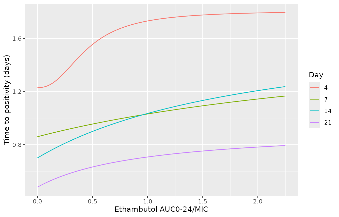
Replicates Figure 4A of Gumbo 2026: time-to-positivity versus AUC0-24/MIC by sampling day (Table 2 parameters).
ggplot(curves, aes(x, log_cfu, colour = day)) +
  geom_line() +
  geom_hline(yintercept = 5.3, linetype = "dotted") +
  coord_cartesian(ylim = c(0, 9)) +
  labs(x = "Ethambutol AUC0-24/MIC", y = "log10 CFU/mL", colour = "Day")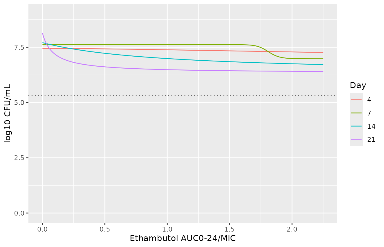
Replicates Figure 4B of Gumbo 2026: total M. kansasii burden versus AUC0-24/MIC by sampling day (Table 2 parameters). Dotted line: B0.
The day-4 and day-7 TTP curves and the day-7 and day-21 CFU curves match the published panels. Several published curves do not follow from the printed Table 2 values. The day-4 and day-14 CFU curves in Figure 4B drop steeply near AUC0-24/MIC 1.75 and plateau about 0.6 log10 below control. The day-14 and day-21 TTP curves in Figure 4A rise as steps near 0.5. Table 2 instead gives EC50s of 3.84 and 0.97 with H = 1.6 and 1.0 (CFU), and EC50s of 2.10 and 0.98 with H = 1.0 (TTP). The package follows Table 2, because the paper’s text reproduces it independently: the mean EC80 of 5.47 and both EC50 coefficients of variation follow from the table above, not from the plotted curves.
ggplot(curves, aes(x, log_cfu_res, colour = day)) +
  geom_line() +
  coord_cartesian(ylim = c(0, 9)) +
  labs(x = "Ethambutol AUC0-24/MIC", y = "Resistant log10 CFU/mL", colour = "Day")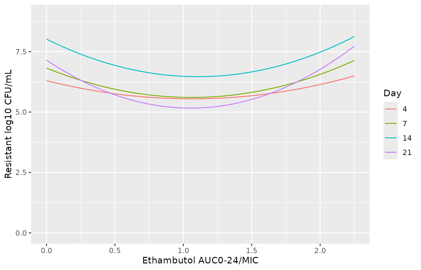
Replicates Figure 4C of Gumbo 2026: ethambutol-resistant subpopulation versus AUC0-24/MIC by sampling day (quadratics digitised from the published curves).
The quadratics bottom out near AUC0-24/MIC 1.05 on every day. Their minima are about 5.6 (days 4 and 7), 6.5 (day 14) and 5.2 (day 21) log10 CFU/mL, matching the “U” shapes of Figure 4C. The paper notes the smallest day-21 resistant subpopulation at 5.18 log10 CFU/mL (Figure 3F, regimen R4, AUC0-24/MIC 1.41). The day-21 quadratic gives the value below at that exposure. R4 is not among the six exposures plotted in Figure 4, so this is an out-of-sample comparison.
r4 <- solve_hfs(data.frame(
  id = 1L, time = 21, evid = 0L, cmt = NA_integer_, dvid = 1L,
  AUC_ETHAMBUTOL = 1.41 * 8
))
r4[, c("log_cfu", "log_cfu_res", "ttp")]
#>    log_cfu log_cfu_res       ttp
#> 1 6.444356    5.392999 0.7454812
Assumptions and deviations
- Cavity-centre layer not included. Gumbo 2026 linked the blood compartment to the air-caseum interface through the dynamical sink model of Dheda et al. 2018 (Am J Respir Crit Care Med 198:1208-1219). That paper fits ethambutol AUC against distance from the blood vessel, and it gives its parameters only in an online data supplement that could not be retrieved when this article was written. Gumbo 2026 prints the sink equation but not its ethambutol parameters (cavity potential energy Xmax, sink centre c0, radius r, steepness nu and the rate constants). The packaged PK model therefore predicts plasma concentrations. It does not reproduce the cavity-centre AUCs of Figure 5A or the probability-of-target-attainment results of Figures 5B-5D, which also depend on the 587-isolate MIC distribution of Table 1.
- IIV as coefficient of variation. The Methods print each IIV as a percentage (“parameters and variances (%)”). It is encoded as the CV of a log-normal distribution, omega^2 = log(1 + CV^2). The paper does not state the distribution used inside ADAPT 5. The whiskers of Figure 5A (minimum and maximum of 10,000 subjects) are narrower than a 34% log-normal CV on clearance would give in plasma. That may reflect the sink layer or a different prior distribution, and it cannot be resolved without the sink parameters.
- Bioavailability. Doses are oral and no bioavailability is given, so CL, Vc, Q and Vp are apparent (relative to F) values, and the dose enters the depot unscaled.
- No residual error. Neither model reports residual variability, so all residual SDs are fixed at 0 and both models are for typical-value or between-subject simulation.
- HFS model is defined only at the sampling days and the tested exposures. The authors fitted each sampling day separately. The packaged model picks the day’s parameter set from the simulation time (cut points at 5.5, 10.5 and 17.5 days), so values between sampling days are a step function, not an interpolation. Predictions beyond AUC0-24/MIC 2.07 extrapolate the Emax curves and, for the resistant subpopulation, a quadratic that rises without bound.
- Resistant-subpopulation coefficients are digitised. Gumbo 2026 does not tabulate the quadratic coefficients. They were obtained by a quadratic least-squares fit to the pixels of each curve in Figure 4C, with axes calibrated on the printed tick marks, and are given to two decimals.
- Figure 4D not encoded. The resistant fraction as a percentage of the total population (Figure 4D) was regressed separately. On day 14 it is flat at 100%, and on day 21 it rises to 100% by AUC0-24/MIC 0.5 and then falls, a shape that is not a quadratic in AUC0-24/MIC. A rough resistant fraction can be formed as 100 x 10^(log_cfu_res - log_cfu), but it will not match the published Figure 4D curves.
-
Absolute AUC plus MIC. Exposure is carried as the
daily AUC (
AUC_ETHAMBUTOL, mg*h/L) divided by the strain MIC of 8 mg/L, not as a ratio column. The HFS AUC0-24 values in Figure 2B equal 8 x the printed AUC0-24/MIC for all six regimens, so the split is exact.