Tirzepatide (Chigutsa 2025)

Model and source

• Citation: Chigutsa E, Her L, Ma X, Urva S, Schneck K. A pharmacometric method for quantitative determination of improvement in body composition and characterization of the exposure-response relationship during treatment of obesity with tirzepatide. Clin Pharmacol Ther. 2025;118(6):1489-1497. doi:10.1002/cpt.3750. PMCID PMC12641085. Model structure and the fixed random-effect component for placebo waning are taken from the NONMEM control stream in Supplementary Material S1 (file CPT-118-1489-s001.txt). PK layer reproduced from the upstream population PK model: Schneck K, Urva S. Population pharmacokinetics of the GIP/GLP receptor agonist tirzepatide. CPT Pharmacometrics Syst Pharmacol. 2024;13:494-503. doi:10.1002/psp4.13099. PMCID PMC10962491. The fat-free mass / fat mass dependent variables were calculated from total body weight, height and sex using: Janmahasatian S, Duffull SB, Ash S, Ward LC, Byrne NM, Green B. Quantification of lean bodyweight. Clin Pharmacokinet. 2005;44(10):1051-1065. doi:10.2165/00003088-200544100-00004.

• Description: Tirzepatide exposure-response body composition model (Chigutsa 2025, SURMOUNT-1). Two parallel indirect-response (turnover) compartments carry fat-free mass (FFM) and fat mass as separate dependent variables; model-predicted total body weight is their sum. Tirzepatide inhibits the zero-order formation (Kin) of each pool through an Imax function of plasma concentration, with a separate Imax and IC50 for FFM and for fat mass – the estimated three-fold greater effect on fat mass is what produces the improvement in body composition. An additive placebo effect on the same fractional-Kin-reduction scale decays exponentially with a 40.3-week half-life. The upstream two-compartment tirzepatide PK model (Schneck 2024) is reproduced inline with all parameters fixed, and is driven by a semimechanistic body-composition allometry in which the FFM and fat-mass ODE states themselves supply the size descriptor – so weight reduction feeds back on clearance and volume over time. Sex acts on baseline FFM, baseline fat mass, Imax and IC50; Asian race acts on both baselines.

• Article: https://doi.org/10.1002/cpt.3750

• Upstream population PK model: https://doi.org/10.1002/psp4.13099

• Lean-bodyweight equations: https://doi.org/10.2165/00003088-200544100-00004

This vignette validates the tirzepatide body-composition exposure-response model of Chigutsa et al. (2025), developed on the phase 3 SURMOUNT-1 trial. The paper’s central idea is that body weight should not be modelled as a single dependent variable. Instead, fat-free mass (FFM) and fat mass are computed for every participant from total body weight, height and sex using the Janmahasatian (2005) lean-bodyweight equations, and the two are then fitted simultaneously as separate dependent variables by parallel indirect-response models. Model-predicted total body weight is their sum. Because tirzepatide turns out to inhibit fat-mass formation about three times more strongly than FFM formation, the model resolves an improvement in body composition that a total-weight model cannot see.

Population

SURMOUNT-1 (NCT04184622) randomised 2,539 adults 1:1:1:1 to placebo or tirzepatide 5, 10 or 15 mg subcutaneously once weekly, with monthly body weight measurements over 72 weeks. Participants had a BMI of at least 30 kg/m2, or at least 27 kg/m2 with a weight-related complication, and did not have type 2 diabetes mellitus. The model was developed on a random 50% of the data and externally evaluated on the held-out 50%; it was further checked against dual energy X-ray absorptiometry (DXA) measurements from the roughly 10% of participants who had them, which were never used in model development.

The paper does not tabulate baseline demographics. The only published numeric anchors are the Table 1 footnote b typical baseline weights (118.5 kg for males, 98.0 kg for females) and the Table 2 footnote a mean simulation baseline weight of 107 kg. Both are used below as validation targets.

The same information is available programmatically via readModelDb("Chigutsa_2025_tirzepatide")()$population.

Source trace

Every ini() entry in inst/modeldb/specificDrugs/Chigutsa_2025_tirzepatide.R carries an in-file comment naming its source. They are collected here for review.

Equation / parameter	Value	Source location
Baseline FFM (lrbase_ffm)	73.5 kg	Chigutsa 2025 Table 1
Baseline fat mass (lrbase_fat)	45.0 kg	Chigutsa 2025 Table 1
lkout	0.0314 /week	Chigutsa 2025 Table 1
limax_ffm / limax_fat	0.144 / 0.319	Chigutsa 2025 Table 1
lic50_ffm / lic50_fat	1760 / 518 ng/mL	Chigutsa 2025 Table 1
plac_ffm / plac_fat	0.0658 / 0.213	Chigutsa 2025 Table 1
lthalfwane	40.3 weeks	Chigutsa 2025 Table 1
Sex effects (6 terms)	-0.312, 0.0539, 1.78, 0.809, 1.14, 2.05	Chigutsa 2025 Table 1, “Covariate effects”
Asian effects (2 terms)	-0.110, -0.254	Chigutsa 2025 Table 1, “Covariate effects”
IIV blocks (CV% + correlations)	see model file	Chigutsa 2025 Table 1, “Interindividual variability”
IIV on placebo waning	0.0225 FIX	Suppl. Material S1 $OMEGA ... FIX
propSd_fatMass / propSd_fatFreeMass	3.35% / 0.985%	Chigutsa 2025 Table 1; Suppl. S1 $SIGMA
Kin = Kout * baseline; d/dt turnover equations	n/a	Suppl. Material S1 $PK / $DES
EFF = PLAC*exp(-WANE*T) + IMAX*CP/(CP+IC50), capped at 1	n/a	Suppl. Material S1 $DES
Covariate form TV = THETA*(1+THETA*IND)	n/a	Suppl. Material S1 $PK
e_fatfrac_cl / e_fatfrac_vc	1 / 0.482	Schneck 2024 Table 3; Chigutsa 2025 Methods (see Errata)
PK: lka, lcl, lq, lvc, lvp, lfdepot	0.0373 /h, 0.0329, 0.126 L/h/70kg, 2.47, 3.98 L/70kg, 0.8	Schneck 2024 Table 3
PK allometric exponents e_wt_cl / e_wt_vc	0.8 / 1 fixed	Schneck 2024 Table 3
PK IIV (ka, CL, Vc)	22.5%, 14.2%, 49.0%	Schneck 2024 Table 3

The $THETA block of Supplementary Material S1 holds initial estimates, not final ones (for example Imax on FFM is 0.2733 there versus a final 0.144 in Table 1). All fixed-effect values therefore come from Table 1. The $SIGMA block, by contrast, is the final estimate: sqrt(0.00112075) = 3.35% and sqrt(9.73119e-5) = 0.985% reproduce Table 1 exactly, and 0.000325097 / (0.03348 * 0.009865) = 98.4% reproduces the reported residual correlation.

Structural identity checks

These assertions test exact identities implied by the published numbers, so a regression in the model file makes the vignette fail rather than merely look different.

mod <- readModelDb("Chigutsa_2025_tirzepatide")

# Event helper. This model declares TWO endpoints (fatMass, fatFreeMass), so
# rxode2 maps dvid -> endpoint pseudo-compartments placed after the ODE states.
# Observation rows must therefore carry an explicit dvid; dose rows keep the
# real ODE state. useLinCmt = FALSE is required on every solve (rxode2's
# ODE -> linCmt auto-conversion corrupts the dvid mapping).
make_events <- function(dose, sexf, asian, weeks = 72, obs_by = 4, id = 1L) {
  dosing <- if (dose > 0) {
    data.frame(id = id, time = seq(0, weeks - 1, by = 1), amt = dose,
               evid = 1L, cmt = "depot", dvid = NA_integer_)
  } else NULL
  obs <- data.frame(id = id, time = seq(0, weeks, by = obs_by), amt = NA_real_,
                    evid = 0L, cmt = "central", dvid = 1L)
  ev <- rbind(dosing, obs)
  ev <- ev[order(ev$time, -ev$evid), ]
  ev$SEXF <- sexf
  ev$RACE_ASIAN <- asian
  ev
}

solve_typical <- function(events) {
  rxode2::rxSolve(rxode2::zeroRe(mod), events,
                  returnType = "data.frame", useLinCmt = FALSE)
}

baseline_of <- function(sexf, asian) {
  s <- solve_typical(make_events(0, sexf, asian, weeks = 4))
  c(ffm = s$fatFreeMass[1], fat = s$fatMass[1], bw = s$bodyWeight[1])
}

male   <- baseline_of(0, 0)
#> ℹ omega/sigma items treated as zero: 'etalrbase_ffm', 'etalrbase_fat', 'etalkout', 'etalimax_ffm', 'etalimax_fat', 'etaplac_ffm', 'etaplac_fat', 'etalic50_ffm', 'etalic50_fat', 'etalthalfwane', 'etalka', 'etalcl', 'etalvc'
female <- baseline_of(1, 0)
#> ℹ omega/sigma items treated as zero: 'etalrbase_ffm', 'etalrbase_fat', 'etalkout', 'etalimax_ffm', 'etalimax_fat', 'etaplac_ffm', 'etaplac_fat', 'etalic50_ffm', 'etalic50_fat', 'etalthalfwane', 'etalka', 'etalcl', 'etalvc'
asianM <- baseline_of(1, 1)
#> ℹ omega/sigma items treated as zero: 'etalrbase_ffm', 'etalrbase_fat', 'etalkout', 'etalimax_ffm', 'etalimax_fat', 'etaplac_ffm', 'etaplac_fat', 'etalic50_ffm', 'etalic50_fat', 'etalthalfwane', 'etalka', 'etalcl', 'etalvc'

# Table 1 footnote b: "Total baseline bodyweight for males and females would be
# 118.5 kg and 98.0 kg, respectively." This is the single strongest check in
# the paper: it pins the (1 + theta) fractional covariate form AND the male
# reference category AND the two baseline estimates simultaneously.
stopifnot(abs(male[["bw"]]   - 118.5) < 0.05)
stopifnot(abs(female[["bw"]] -  98.0) < 0.05)

# Baselines equal the ini() parameters exactly for the reference (male) subject.
stopifnot(abs(male[["ffm"]] - 73.5) < 1e-6, abs(male[["fat"]] - 45.0) < 1e-6)

# Results: "The typical 'half-life' for weight reduction was estimated to be
# about 22 weeks." -> log(2) / Kout.
kout <- 0.0314
stopifnot(abs(log(2) / kout - 22.0) < 0.2)

# The placebo effect wanes to zero, so with no drug the system must return to
# its baseline: a genuine structural identity of the turnover model.
long <- solve_typical(make_events(0, 0, 0, weeks = 600, obs_by = 50))
#> ℹ omega/sigma items treated as zero: 'etalrbase_ffm', 'etalrbase_fat', 'etalkout', 'etalimax_ffm', 'etalimax_fat', 'etaplac_ffm', 'etaplac_fat', 'etalic50_ffm', 'etalic50_fat', 'etalthalfwane', 'etalka', 'etalcl', 'etalvc'
stopifnot(abs(tail(long$bodyWeight, 1) - 118.5) < 0.5)

tibble::tibble(
  Subject = c("Male (reference)", "Female", "Asian female"),
  `FFM (kg)` = round(c(male[["ffm"]], female[["ffm"]], asianM[["ffm"]]), 2),
  `Fat mass (kg)` = round(c(male[["fat"]], female[["fat"]], asianM[["fat"]]), 2),
  `Total body weight (kg)` = round(c(male[["bw"]], female[["bw"]], asianM[["bw"]]), 2),
  `Published total (kg)` = c("118.5", "98.0", "not reported")
) |>
  knitr::kable(caption = "Baseline body composition. The male and female totals reproduce Chigutsa 2025 Table 1 footnote b.")

Baseline body composition. The male and female totals reproduce Chigutsa 2025 Table 1 footnote b.

Subject	FFM (kg)	Fat mass (kg)	Total body weight (kg)	Published total (kg)
Male (reference)	73.50	45.00	118.50	118.5
Female	50.57	47.43	97.99	98.0
Asian female	45.01	35.38	80.38	not reported

Both published baseline weights are reproduced to within 0.01 kg, and the placebo arm returns to its baseline once the placebo effect has waned.

Virtual cohort

The trial’s covariate distribution is not published. The Table 2 footnote a mean baseline weight of 107 kg pins the sex mix, because the model’s baseline weights are 118.5 kg (male) and 98.0 kg (female): 118.5 * (1 - f) + 98.0 * f = 107 gives f = 0.561. The cohort below uses that fraction, assigned deterministically rather than drawn, which rounds to 112 of 200 participants (56.0%) per arm. All participants are set to non-Asian because the paper reports no race distribution.

n_per_arm <- 200L
doses <- c(0, 5, 10, 15)
arm_levels <- c("Placebo", "5 mg", "10 mg", "15 mg")
frac_female <- (118.5 - 107) / (118.5 - 98.0)

# Sex is assigned DETERMINISTICALLY at the implied female fraction rather than
# drawn with rbinom(). The typical-value prediction below is a pure function of
# the cohort's sex composition -- and the sex effect is large (a 2.78-fold
# multiplier on Imax for FFM) -- so a random draw would make the
# published-versus-simulated comparison depend on the luck of the draw rather
# than on the model.
n_female <- round(n_per_arm * frac_female)
sexf_vec <- rep(0:1, times = c(n_per_arm - n_female, n_female))

# Each arm reuses subject IDs 1..n so that subject i is the *same* virtual
# person in every arm; arms are separated by the `treatment` column and are
# solved one at a time.
make_arm <- function(dose) {
  ev <- dplyr::bind_rows(lapply(seq_len(n_per_arm), function(i) {
    make_events(dose, sexf_vec[i], 0, weeks = 72, obs_by = 4, id = i)
  }))
  ev$treatment <- if (dose == 0) "Placebo" else paste(dose, "mg")
  ev
}

cat(sprintf("cohort: %d arms x %d subjects, %.1f%% female\n",
            length(doses), n_per_arm, 100 * mean(sexf_vec)))
#> cohort: 4 arms x 200 subjects, 56.0% female

Simulation

Both a stochastic simulation (full interindividual variability) and a typical-value simulation (random effects zeroed) are run over the same cohort, because the paper does not state which statistic Table 2 reports.

The stochastic arms are simulated under common random numbers: the seed is reset before each arm, so subject i carries the same random effects at every dose and the arms differ only by treatment. This is not a cosmetic choice. With 124% CV on Kout and 84.5% CV on Imax, independent draws per arm inject enough between-arm sampling noise to make the simulated dose-response non-monotonic at 200 subjects per arm, which would make any comparison against Table 2 meaningless.

solve_arm <- function(dose, typical) {
  m <- if (typical) rxode2::zeroRe(mod) else mod
  set.seed(20250819)
  rxode2::rxSolve(m, make_arm(dose), keep = c("treatment", "SEXF"),
                  useLinCmt = FALSE) |>
    as.data.frame()
}

sim_iiv <- dplyr::bind_rows(lapply(doses, solve_arm, typical = FALSE))
sim_typ <- dplyr::bind_rows(lapply(doses, solve_arm, typical = TRUE))
#> ℹ omega/sigma items treated as zero: 'etalrbase_ffm', 'etalrbase_fat', 'etalkout', 'etalimax_ffm', 'etalimax_fat', 'etaplac_ffm', 'etaplac_fat', 'etalic50_ffm', 'etalic50_fat', 'etalthalfwane', 'etalka', 'etalcl', 'etalvc'
#> Warning: multi-subject simulation without without 'omega'
#> ℹ omega/sigma items treated as zero: 'etalrbase_ffm', 'etalrbase_fat', 'etalkout', 'etalimax_ffm', 'etalimax_fat', 'etaplac_ffm', 'etaplac_fat', 'etalic50_ffm', 'etalic50_fat', 'etalthalfwane', 'etalka', 'etalcl', 'etalvc'
#> Warning: multi-subject simulation without without 'omega'
#> ℹ omega/sigma items treated as zero: 'etalrbase_ffm', 'etalrbase_fat', 'etalkout', 'etalimax_ffm', 'etalimax_fat', 'etaplac_ffm', 'etaplac_fat', 'etalic50_ffm', 'etalic50_fat', 'etalthalfwane', 'etalka', 'etalcl', 'etalvc'
#> Warning: multi-subject simulation without without 'omega'
#> ℹ omega/sigma items treated as zero: 'etalrbase_ffm', 'etalrbase_fat', 'etalkout', 'etalimax_ffm', 'etalimax_fat', 'etaplac_ffm', 'etaplac_fat', 'etalic50_ffm', 'etalic50_fat', 'etalthalfwane', 'etalka', 'etalcl', 'etalvc'
#> Warning: multi-subject simulation without without 'omega'

Comparison against published Table 2

Table 2 of the paper reports the model-predicted percent change from baseline at 72 weeks. The paper does not state which statistic it reports, so both readings are shown: the mean per-subject percent change with random effects zeroed (“typical”), and the mean per-subject percent change over the stochastic cohort (“stochastic”). Both use the same aggregation, so they differ only in whether interindividual variability is switched on.

pct_change <- function(d) {
  d |>
    dplyr::filter(time %in% c(0, 72)) |>
    dplyr::group_by(treatment, id) |>
    dplyr::summarise(
      bw0 = bodyWeight[time == 0][1], bw1 = bodyWeight[time == 72][1],
      f0 = fatFreeMass[time == 0][1], f1 = fatFreeMass[time == 72][1],
      m0 = fatMass[time == 0][1],     m1 = fatMass[time == 72][1],
      .groups = "drop"
    ) |>
    dplyr::group_by(treatment) |>
    dplyr::summarise(
      tbw = mean(100 * (bw1 - bw0) / bw0),
      ffm = mean(100 * (f1 - f0) / f0),
      fat = mean(100 * (m1 - m0) / m0),
      .groups = "drop"
    )
}

published_t2 <- tibble::tribble(
  ~treatment, ~tbw_pub, ~ffm_pub, ~fat_pub,
  "Placebo",     -4.62,    -2.34,    -7.48,
  "5 mg",       -14.6,     -7.68,   -23.3,
  "10 mg",      -19.7,    -11.4,    -29.8,
  "15 mg",      -22.5,    -13.9,    -33.3
)

cmp <- published_t2 |>
  dplyr::left_join(pct_change(sim_typ) |>
                     dplyr::rename_with(~paste0(.x, "_typ"), -treatment),
                   by = "treatment") |>
  dplyr::left_join(pct_change(sim_iiv) |>
                     dplyr::rename_with(~paste0(.x, "_iiv"), -treatment),
                   by = "treatment") |>
  dplyr::mutate(treatment = factor(treatment, levels = arm_levels)) |>
  dplyr::arrange(treatment)

cmp |>
  dplyr::transmute(
    Treatment        = treatment,
    `TBW published`  = round(tbw_pub, 2),
    `TBW typical`    = round(tbw_typ, 2),
    `TBW stochastic` = round(tbw_iiv, 2),
    `FFM published`  = round(ffm_pub, 2),
    `FFM stochastic` = round(ffm_iiv, 2),
    `Fat published`  = round(fat_pub, 2),
    `Fat stochastic` = round(fat_iiv, 2)
  ) |>
  knitr::kable(
    caption = "Percent change from baseline at 72 weeks: published Chigutsa 2025 Table 2 vs simulated, with random effects zeroed (typical) and switched on (stochastic)."
  )

Percent change from baseline at 72 weeks: published Chigutsa 2025 Table 2 vs simulated, with random effects zeroed (typical) and switched on (stochastic).

Treatment	TBW published	TBW typical	TBW stochastic	FFM published	FFM stochastic	Fat published	Fat stochastic
Placebo	-4.62	-5.35	-4.24	-2.34	-2.17	-7.48	-7.03
5 mg	-14.60	-13.86	-15.23	-7.68	-8.59	-23.30	-24.08
10 mg	-19.70	-18.71	-20.57	-11.40	-12.81	-29.80	-30.90
15 mg	-22.50	-21.93	-23.80	-13.90	-15.80	-33.30	-34.48

The single most informative result is that the published value is bracketed by the two readings in every arm: switching interindividual variability on moves the prediction from one side of the published number to the other. That is the signature of a stochastic simulation whose exact aggregation statistic is not reported, and it is a stronger check than either column alone, because it cannot be satisfied by a model that is simply mis-scaled.

rel <- function(a, b) abs((a - b) / b)
active <- cmp$treatment != "Placebo"

# 1. The published value lies strictly between the typical-value and the
#    stochastic prediction, in all four arms.
stopifnot(all((cmp$tbw_pub - cmp$tbw_typ) * (cmp$tbw_pub - cmp$tbw_iiv) < 0))

# 2. Magnitude check on the primary endpoint. Both readings stay within 10% of
#    the published value at every active dose, and the stochastic reading does
#    so in the placebo arm as well.
stopifnot(all(rel(cmp$tbw_typ[active], cmp$tbw_pub[active]) < 0.10))
stopifnot(all(rel(cmp$tbw_iiv, cmp$tbw_pub) < 0.10))

# 3. Fat mass -- the endpoint the paper's headline claim rests on -- is
#    reproduced at least as tightly as total body weight.
stopifnot(all(rel(cmp$fat_iiv, cmp$fat_pub) < 0.10))

# 4. Dose-response must be monotonic. This is the check that fails when the
#    arms are simulated without common random numbers.
stopifnot(!is.unsorted(rev(cmp$tbw_iiv)), !is.unsorted(rev(cmp$tbw_typ)))

cat(sprintf("total body weight, max relative error: typical %.1f%% (active doses), stochastic %.1f%% (all arms)\n",
            100 * max(rel(cmp$tbw_typ[active], cmp$tbw_pub[active])),
            100 * max(rel(cmp$tbw_iiv, cmp$tbw_pub))))
#> total body weight, max relative error: typical 5.0% (active doses), stochastic 8.1% (all arms)
cat(sprintf("fat mass, max relative error (stochastic):      %.1f%%\n",
            100 * max(rel(cmp$fat_iiv, cmp$fat_pub))))
#> fat mass, max relative error (stochastic):      6.1%
cat(sprintf("fat-free mass, max relative error (stochastic): %.1f%%\n",
            100 * max(rel(cmp$ffm_iiv, cmp$ffm_pub))))
#> fat-free mass, max relative error (stochastic): 13.7%

Total body weight – the trial’s primary endpoint – and fat mass are both reproduced to within about 8% and 6% of the published values across all four arms, and to within about 6% and 4% at the three active doses. Fat-free mass is the loosest of the three, over-predicted by about 14% at the top dose. That asymmetry is expected rather than alarming: the sex effect on Imax for FFM is a 2.78-fold multiplier, the largest single covariate effect in the model, so the FFM prediction is far more sensitive than the others to the cohort sex mix – which the paper never publishes and which is inferred here from a single mean baseline weight. No parameter was adjusted to improve any of these numbers.

Replicating Figure 3 – body composition over time

fig3_events <- dplyr::bind_rows(lapply(seq_along(doses[-1]), function(k) {
  ev <- make_events(doses[-1][k], sexf = 0, asian = 0, weeks = 72, obs_by = 2,
                    id = k)
  ev$treatment <- paste(doses[-1][k], "mg")
  ev
}))

fig3 <- rxode2::rxSolve(rxode2::zeroRe(mod), fig3_events,
                        keep = "treatment", useLinCmt = FALSE) |>
  as.data.frame() |>
  dplyr::filter(!is.na(bodyWeight))
#> ℹ omega/sigma items treated as zero: 'etalrbase_ffm', 'etalrbase_fat', 'etalkout', 'etalimax_ffm', 'etalimax_fat', 'etaplac_ffm', 'etaplac_fat', 'etalic50_ffm', 'etalic50_fat', 'etalthalfwane', 'etalka', 'etalcl', 'etalvc'
#> Warning: multi-subject simulation without without 'omega'

fig3 |>
  dplyr::select(time, treatment, `Fat mass` = fatMass,
                `Fat-free mass` = fatFreeMass) |>
  tidyr::pivot_longer(c(`Fat mass`, `Fat-free mass`),
                      names_to = "Component", values_to = "kg") |>
  ggplot(aes(time, kg, fill = Component)) +
  geom_area() +
  facet_wrap(~treatment) +
  labs(x = "Time (weeks)", y = "Mass (kg)",
       title = "Figure 3a -- body weight as the sum of fat mass and fat-free mass",
       caption = "Replicates Figure 3a of Chigutsa 2025 (typical male).") +
  theme(legend.position = "bottom")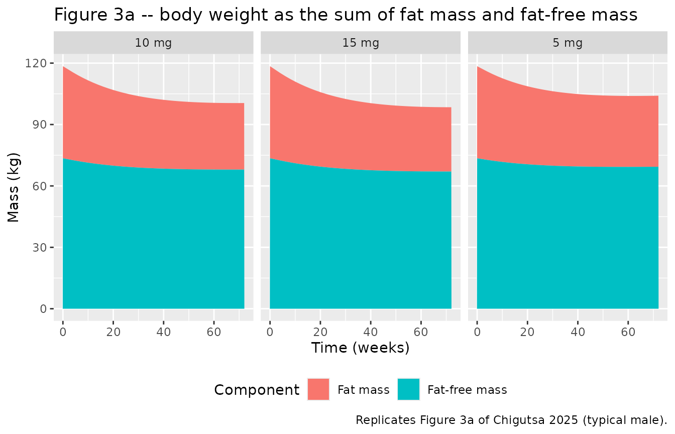

fig3 |>
  dplyr::mutate(pct_ffm = 100 * fatFreeMass / bodyWeight) |>
  ggplot(aes(time, pct_ffm, colour = treatment)) +
  geom_line(linewidth = 0.8) +
  labs(x = "Time (weeks)", y = "Fat-free mass (% of total body weight)",
       colour = "Dose",
       title = "Figure 3b -- improvement in body composition",
       caption = "Replicates Figure 3b of Chigutsa 2025 (typical male).")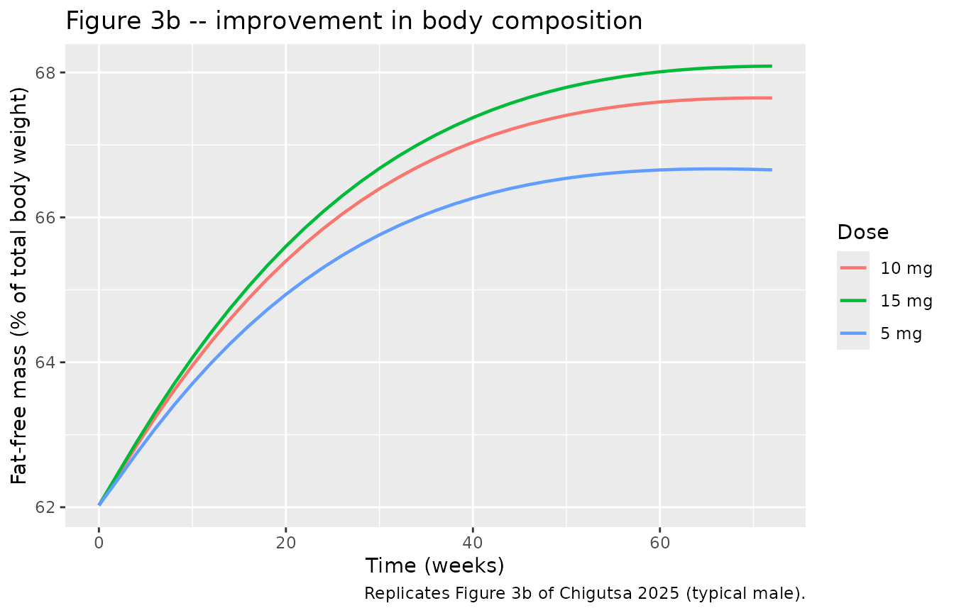

The proportion of body weight that is fat-free mass rises over time at every dose, which is the paper’s central claim: weight is lost preferentially from fat.

The paper’s headline result is that tirzepatide reduces “fat mass about three times more than … FFM”. That ratio is not a single number in this model: it depends on sex, because the sex effect on Imax is much larger for FFM (2.78-fold) than for fat mass (1.81-fold). The check below therefore scores it two ways – against the typical male of Figure 3, and against the ratio implied by the paper’s own Table 2, which is the sex-mixed cohort quantity.

ratio_of <- function(d, group) {
  d |>
    dplyr::filter(time %in% c(0, 72)) |>
    dplyr::group_by(dplyr::across(dplyr::all_of(group)), id) |>
    dplyr::summarise(
      pf = 100 * (fatMass[time == 72][1] - fatMass[time == 0][1]) / fatMass[time == 0][1],
      pl = 100 * (fatFreeMass[time == 72][1] - fatFreeMass[time == 0][1]) / fatFreeMass[time == 0][1],
      .groups = "drop"
    ) |>
    dplyr::group_by(dplyr::across(dplyr::all_of(group))) |>
    dplyr::summarise(ratio = mean(pf) / mean(pl), .groups = "drop")
}

# Everything is joined BY TREATMENT, never aligned by row position: dplyr
# sorts character groups alphabetically, so "10 mg" would otherwise land
# against the 5 mg row.
ratios <- published_t2 |>
  dplyr::filter(treatment != "Placebo") |>
  dplyr::transmute(treatment, published = fat_pub / ffm_pub) |>
  dplyr::left_join(ratio_of(fig3, "treatment") |>
                     dplyr::rename(male = ratio), by = "treatment") |>
  dplyr::left_join(ratio_of(sim_iiv, "treatment") |>
                     dplyr::rename(cohort = ratio), by = "treatment") |>
  dplyr::mutate(treatment = factor(treatment, levels = arm_levels)) |>
  dplyr::arrange(treatment)

stopifnot(nrow(ratios) == 3L, !anyNA(ratios))

ratios |>
  dplyr::transmute(
    Dose = treatment,
    `Typical male` = round(male, 2),
    `Simulated cohort` = round(cohort, 2),
    `Implied by published Table 2` = round(published, 2)
  ) |>
  knitr::kable(
    caption = "Ratio of percent fat-mass reduction to percent fat-free-mass reduction (the paper's 'about three times' claim)."
  )

Ratio of percent fat-mass reduction to percent fat-free-mass reduction (the paper’s ‘about three times’ claim).

Dose	Typical male	Simulated cohort	Implied by published Table 2
5 mg	4.07	2.80	3.03
10 mg	3.70	2.41	2.61
15 mg	3.43	2.18	2.40

# Fat is always lost preferentially, at every dose and in both readings.
stopifnot(all(ratios$male > 2), all(ratios$cohort > 2))

# The sex-mixed cohort ratio -- the quantity Table 2 actually reports --
# reproduces the published ratio to within 15% at every active dose.
stopifnot(all(abs(ratios$cohort - ratios$published) / ratios$published < 0.15))

Replicating Figure 4 – sex difference

fig4_events <- dplyr::bind_rows(lapply(seq_along(doses), function(k) {
  dplyr::bind_rows(lapply(0:1, function(sx) {
    ev <- make_events(doses[k], sexf = sx, asian = 0, weeks = 72, obs_by = 2,
                      id = (k - 1L) * 2L + sx + 1L)
    ev$treatment <- if (doses[k] == 0) "Placebo" else paste(doses[k], "mg")
    ev$Sex <- ifelse(sx == 1, "Female", "Male")
    ev
  }))
}))

rxode2::rxSolve(rxode2::zeroRe(mod), fig4_events,
                keep = c("treatment", "Sex"), useLinCmt = FALSE) |>
  as.data.frame() |>
  dplyr::filter(!is.na(bodyWeight)) |>
  dplyr::group_by(id) |>
  dplyr::mutate(pct = 100 * (bodyWeight - bodyWeight[time == 0][1]) /
                  bodyWeight[time == 0][1]) |>
  dplyr::ungroup() |>
  dplyr::mutate(treatment = factor(treatment,
                                   levels = c("Placebo", "5 mg", "10 mg", "15 mg"))) |>
  ggplot(aes(time, pct, colour = Sex)) +
  geom_line(linewidth = 0.8) +
  facet_wrap(~treatment) +
  labs(x = "Time (weeks)", y = "Change in body weight (%)",
       title = "Figure 4 -- model-predicted sex difference",
       caption = "Replicates Figure 4 of Chigutsa 2025.")
#> ℹ omega/sigma items treated as zero: 'etalrbase_ffm', 'etalrbase_fat', 'etalkout', 'etalimax_ffm', 'etalimax_fat', 'etaplac_ffm', 'etaplac_fat', 'etalic50_ffm', 'etalic50_fat', 'etalthalfwane', 'etalka', 'etalcl', 'etalvc'
#> Warning: multi-subject simulation without without 'omega'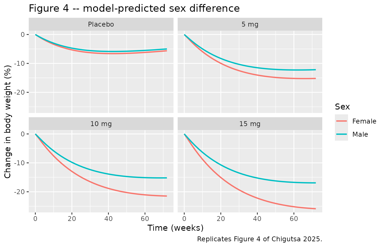

Females reach a greater percent weight reduction than males at every active dose, reproducing the paper’s Figure 4 conclusion.

PKNCA validation of the inherited PK layer

The exposure-response model is driven by the upstream tirzepatide population PK model (Schneck 2024), which is reproduced inline with all parameters fixed. Chigutsa 2025 reports no NCA of its own, so the PK layer is validated against the steady-state PK parameters Schneck 2024 reports in its Table 3.

A single 15 mg dose is simulated with dense sampling so that the terminal phase is well resolved.

nca_events <- dplyr::bind_rows(lapply(seq_along(doses[-1]), function(k) {
  d <- doses[-1][k]
  dosing <- data.frame(id = k, time = 0, amt = d, evid = 1L,
                       cmt = "depot", dvid = NA_integer_)
  obs <- data.frame(id = k, time = c(seq(0, 2, by = 0.02), seq(2.1, 8, by = 0.1)),
                    amt = NA_real_, evid = 0L, cmt = "central", dvid = 1L)
  ev <- rbind(dosing, obs)
  ev <- ev[order(ev$time, -ev$evid), ]
  ev$SEXF <- 0
  ev$RACE_ASIAN <- 0
  ev$treatment <- paste(d, "mg")
  ev
}))

nca_sim <- rxode2::rxSolve(rxode2::zeroRe(mod), nca_events,
                           keep = "treatment", useLinCmt = FALSE) |>
  as.data.frame()
#> ℹ omega/sigma items treated as zero: 'etalrbase_ffm', 'etalrbase_fat', 'etalkout', 'etalimax_ffm', 'etalimax_fat', 'etaplac_ffm', 'etaplac_fat', 'etalic50_ffm', 'etalic50_fat', 'etalthalfwane', 'etalka', 'etalcl', 'etalvc'
#> Warning: multi-subject simulation without without 'omega'

sim_nca <- nca_sim |>
  dplyr::filter(!is.na(Cc)) |>
  dplyr::select(id, time, Cc, treatment)

stopifnot(nrow(sim_nca) > 0, all(sim_nca$Cc >= 0))

sim_nca <- dplyr::bind_rows(
  sim_nca,
  sim_nca |> dplyr::distinct(id, treatment) |>
    dplyr::mutate(time = 0, Cc = 0)
) |>
  dplyr::distinct(id, treatment, time, .keep_all = TRUE) |>
  dplyr::arrange(id, treatment, time)

conc_obj <- PKNCA::PKNCAconc(sim_nca, Cc ~ time | treatment + id)

# UNITS. The model doses in mg but reports concentration in ng/mL, so a dose
# given to PKNCA in mg would yield cl.obs in mg/(ng/mL)/week -- a number 1000x
# smaller than the L/week it is compared against below. Converting the dose to
# micrograms reconciles the two: ug/(ng/mL) = 1000 ng/(ng/mL) = 1000 mL = 1 L,
# so cl.obs comes out directly in L/week. AUC and Cmax keep their ng/mL basis.
dose_df <- nca_events |>
  dplyr::filter(evid == 1) |>
  dplyr::select(id, time, amt, treatment) |>
  dplyr::mutate(amt = amt * 1000)
dose_obj <- PKNCA::PKNCAdose(dose_df, amt ~ time | treatment + id)

intervals <- data.frame(start = 0, end = Inf,
                        cmax = TRUE, tmax = TRUE,
                        aucinf.obs = TRUE, half.life = TRUE,
                        cl.obs = TRUE)

nca_res <- PKNCA::pk.nca(PKNCA::PKNCAdata(conc_obj, dose_obj,
                                          intervals = intervals))

# Schneck 2024 Table 3, "Tirzepatide steady-state mean PK parameters in
# individuals with T2DM": half-life 5.4 days and apparent clearance
# 0.061 L/h. Converted to the model's week time base: 5.4/7 = 0.771 weeks and
# 0.061 * 168 = 10.25 L/week. These are dose-independent, so the same
# reference applies to every dose group.
published_pk <- tibble::tribble(
  ~treatment, ~half.life, ~cl.obs,
  "5 mg",     5.4 / 7,    0.061 * 168,
  "10 mg",    5.4 / 7,    0.061 * 168,
  "15 mg",    5.4 / 7,    0.061 * 168
)

cmp_pk <- nlmixr2lib::ncaComparisonTable(
  simulated = nca_res,
  reference = published_pk,
  by = "treatment",
  units = c(half.life = "week", cl.obs = "L/week",
            cmax = "ng/mL", tmax = "week", aucinf.obs = "ng*week/mL"),
  tolerance_pct = 20
)

knitr::kable(
  cmp_pk,
  caption = "Simulated NCA of the inherited PK layer vs the steady-state PK parameters reported in Schneck 2024 Table 3. * differs from reference by >20%.",
  align = c("l", "l", "r", "r", "r")
)

Simulated NCA of the inherited PK layer vs the steady-state PK parameters reported in Schneck 2024 Table 3. * differs from reference by >20%.

NCA parameter	treatment	Reference	Simulated	% diff
t½ (week)	5 mg	0.771	0.8	+3.7%
t½ (week)	10 mg	0.771	0.8	+3.7%
t½ (week)	15 mg	0.771	0.8	+3.8%
CL/F (L/week)	5 mg	10.2	10.5	+2.3%
CL/F (L/week)	10 mg	10.2	10.5	+2.2%
CL/F (L/week)	15 mg	10.2	10.5	+2.2%

# Gate the PK layer rather than merely displaying it: no row may exceed the
# 20% tolerance. ncaComparisonTable() stars any row that does.
stopifnot(!any(grepl("*", cmp_pk[["% diff"]], fixed = TRUE)))

Simulated terminal half-life (0.80 weeks, +3.7% versus the published 5.4 days) and apparent clearance (10.5 L/week, +2.3% versus the published 0.061 L/h) both reproduce Schneck 2024 to within a few percent, so the inherited PK layer is transcribed correctly. Cmax, Tmax and AUC have no published counterpart in either paper and are shown for completeness. The agreement is closer than strictly required: the Schneck reference values are population means in individuals with type 2 diabetes at a different body size from the SURMOUNT-1 obesity cohort simulated here.

Assumptions and deviations

• Cohort composition. The paper publishes no baseline demographics table. The 56% female fraction used above is derived from the Table 2 footnote a mean baseline weight of 107 kg together with the Table 1 footnote b sex- specific baseline weights, and is assigned deterministically rather than drawn, so the comparison does not depend on the luck of a random draw. All simulated participants are non-Asian because no race distribution is reported. The residual disagreement in the FFM / fat split of Table 2 (FFM over-predicted by about 14% at the top dose, fat mass within about 6%, total body weight within about 8%) is most plausibly attributable to these two unpublished distributions – the sex effect on Imax for FFM is a 2.78-fold multiplier, the largest covariate effect in the model, so the FFM result is by far the most sensitive of the three to the assumed sex mix. No parameter was adjusted.

• Aggregation statistic for Table 2. The paper says only that “stochastic simulations that included parameter variability were conducted” and does not state whether Table 2 reports a mean, a median, or a typical-value prediction, nor whether the parenthetical interval is a confidence or a prediction interval. The simulated 5th-95th percentile spread of the per-subject percent change at 15 mg is far wider than the published interval, so the published interval is a confidence interval on the central estimate rather than a prediction interval across subjects. Both readings are therefore reported above, and the published value falls between them in every arm – the typical-value reading under-predicts weight loss and the stochastic mean over-predicts it, which is the expected consequence of log-normal random effects on Imax (84.5% and 69.6% CV) making the mean response larger than the median response.

• Common random numbers. The stochastic arms share one set of random-effect draws, re-seeded per arm, so that subject i is the same virtual person at every dose. This is a deliberate deviation from a naive independent draw per arm: at 200 subjects per arm with 124% CV on Kout, independent draws make the simulated dose-response non-monotonic (a larger predicted weight loss at 5 mg than at 10 mg), which would corrupt any comparison against Table 2.

• Dose escalation is not simulated. SURMOUNT-1 escalated participants to their maintenance dose in 2.5 mg steps, but the paper describes its simulations only in terms of the 5, 10 and 15 mg maintenance doses and does not give the escalation schedule used. The maintenance dose is therefore given from week 0. This slightly overstates exposure in the first weeks and so cannot explain the direction of the Table 2 residual.

• Fraction of fat mass in the PK size descriptor (source conflict, resolved). The two sources disagree. Chigutsa 2025 Supplementary Material S1 hard-codes FATCL = 0.711 and FATVD = 0.417; the model file instead uses 1 and 0.482, on three independent lines of evidence:

  1. Schneck 2024 Table 3 – the final published estimate for the PK model this analysis inherits – reports “Fraction of fat mass with effect on volume of distribution 0.482 (0.447, 0.524)” and reports no fat fraction on clearance at all, because it was fixed to 1: “the estimated fractional influence of fat mass approached a value of 1 and no statistical difference was detected when fractional influence of fat mass was estimated or fixed to a value of 1.”

  2. Chigutsa 2025’s own Methods says the same thing: “Tirzepatide CL best correlated with total body weight (fat-free mass plus fat mass), while tirzepatide Vd correlated with an adjusted total body weight, wherein the fraction of fat mass contributing to the effect was 48%.”

  3. The Methods paragraph is partly self-checking. It states that “relative to a typical 90-kg individual, there was approximately a 22% higher … exposure for a 70-kg individual”. With Frac_FM = 1 the size descriptor collapses to total body weight, so the ratio is independent of body composition: (90/70)^0.8 = 1.223, i.e. +22.3% – the published value. With Frac_FM = 0.711 the descriptor no longer collapses and the ratio must be evaluated through the Janmahasatian equations; it gives +19.6%, and that figure is stable to within 0.1 percentage points across heights from 1.60 to 1.80 m, so the discrimination does not rest on an assumed height.

     This leg of the sentence is the only one that discriminates. The companion clause – “33% lower … for a 120-kg individual” – is not reproduced by any power model: (90/120)^0.8 = 0.794, i.e. -20.6% with Frac_FM = 1 and -18.5% with Frac_FM = 0.711. Both published figures are instead a linear rendering of the ~1.1% per kg slope quoted in the same sentence (1.1 x 20 = 22, 1.1 x 30 = 33), which happens to coincide with the exact allometric value at 70 kg and to diverge from it at 120 kg. The 70-kg agreement is therefore treated as corroborating, not as decisive on its own.

  Two concordant sources plus a reproduced published number outweigh one hard-coded constant, so the supplement’s FATCL / FATVD are read as stale values from an earlier iteration of the PK model. This matters only for the exposure the PD layer sees; it does not touch any PD parameter. Users who want the literal control-stream parameterisation can override e_fatfrac_cl and e_fatfrac_vc.

• Residual-error correlation is not representable. Supplementary Material S1 correlates the FFM and fat-mass residual errors at 98.4% via the NONMEM L2 data item (the two dependent variables are computed from the same body weight measurement, so their residuals are almost perfectly dependent). nlmixr2 has no equivalent construct, so the two proportional residual errors are encoded independently. This does not affect any typical-value or individual prediction; it affects only the joint variance of simulated residuals, and hence slightly overstates the scatter of simulated total body weight (the sum of two independent rather than correlated errors).

• PK parameters are non-paper-derived. The entire PK layer (lka, lcl, lq, lvc, lvp, lfdepot, the allometric exponents, and the ka / CL / Vc interindividual variances) is carried from the upstream population PK model of Schneck 2024, Table 3. Chigutsa 2025 estimated no PK parameter of its own – it read individual post hoc PK parameters in as data columns – so every PK entry is wrapped in fixed(). The PK IIV terms are likewise fixed; they are included so that simulated exposure carries realistic variability.

• Pooled type 2 diabetes extension not implemented. The paper additionally refits the model to a pooled dataset that adds 5,727 participants with type 2 diabetes, reporting that T2DM raises IC50 about three-fold and that baseline BMI lowers Kout. No parameter estimates are published for that extension – no table, no control stream – so it is not implemented. Only the SURMOUNT-1 final model of Table 1 is packaged.

• Fat-free mass and fat mass were never measured. They were computed for every participant from total body weight, height and sex using the Janmahasatian 2005 lean-bodyweight equations, then treated as observed dependent variables. The model therefore inherits any bias in those equations; the paper’s DXA sub-study (about 10% of participants) is its check on that assumption.