Model and source
#> ℹ parameter labels from comments will be replaced by 'label()'- Citation: Lau C, van Kesteren C, Smeenk RM, Beex-Oosterhuis MM, Koch BCP, Chan LN, Lin YS, van Rongen A, Knibbe CAJ, Huitema ADR, Huisman-Siebinga H. Semi-Physiological Population Pharmacokinetic Modeling of Oral and Intravenous Paracetamol to Quantify Presystemic Metabolism and Enterohepatic Recirculation. CPT Pharmacometrics Syst Pharmacol. 2026;15(3):e70168. doi:10.1002/psp4.70168.
- Article: https://doi.org/10.1002/psp4.70168
- Supplementary Materials 1 (Table S1, drug- and system-specific parameters and equations) and Supplementary Materials 3 (Data S1, the NONMEM control stream) are part of the same open-access deposit.
Semi-physiological popPK. Joint parent-and-metabolites population PK model for oral and intravenous paracetamol (acetaminophen, PCM) and its glucuronide (PCM-GLU), sulphate (PCM-SUL), and combined cysteine + mercapturate (PCM-CYS & PCM-MER) metabolites in adults with and without obesity (Lau 2026). Extends the intravenous-only model of van Rongen 2016 by resolving first-pass loss into its anatomical sites: a well-stirred liver whose three parallel intrinsic clearances (glucuronidation, sulphation, CYP2E1 oxidation) set pathway-specific hepatic extraction ratios against a weight-driven hepatic blood flow, and a gut wall whose intrinsic CYP2E1 clearance (a fixed fraction of the hepatic oxidative intrinsic clearance) sets the gut extraction ratio against Q_gut. Gut wall, portal vein, and liver are quasi-steady-state algebraic pools rather than ODE states, so absorbed and recirculated drug is presented to the liver on every pass while systemic drug is presented at hepatic blood flow. Enterohepatic recirculation routes 10 percent of newly formed PCM-GLU into a gallbladder compartment that empties over two fixed 6-minute windows per study, releasing drug to a reuptake depot that is deglucuronidated and reabsorbed as parent PCM. Lean body mass scales parent volume, glucuronidation and oxidation intrinsic clearances, and glucuronide elimination clearance; total body weight scales glucuronide volume and drives cardiac output. Study-specific multipliers on the oxidative intrinsic clearance and on all three metabolite elimination clearances separate the Chen oral cohort from the other two studies.
Lau 2026 extends the intravenous-only parent-and-metabolites model of
van Rongen 2016 (packaged here as
vanRongen_2016_acetaminophen) so that a single model
describes both oral and intravenous paracetamol. Three structural
additions carry that extension:
-
A well-stirred liver. The three metabolic routes
are re-parameterised from plasma clearances into intrinsic
hepatic clearances (
CL_H,int) acting against a body-weight-driven hepatic blood flow, so each route has its own hepatic extraction ratioE_Hand first-pass loss is resolved explicitly rather than folded into a lumped bioavailability. - An oxidatively metabolising gut wall. The intestinal CYP2E1 intrinsic clearance is estimated as a fixed fraction (0.00474) of the hepatic oxidative intrinsic clearance and produces PCM-CYS & PCM-MER presystemically. Lau 2026 reports this as the first description of intestinal oxidative metabolism.
- Enterohepatic recirculation of the glucuronide. Ten percent of newly formed PCM-GLU is routed to a gallbladder compartment that empties over two 6-minute windows at study-specific times, delivering drug to a reuptake pool that is deglucuronidated and reabsorbed as parent paracetamol.
Gut wall, portal vein and liver are quasi-steady-state algebraic pools, not ODE states: each pool’s amount is set so its outflow matches its inflow at every instant. That is how the deposited control stream writes them, and it is what makes the model semi-physiological rather than a full PBPK.
Population
| Field | Value |
|---|---|
| species | human |
| n_subjects | 69 |
| n_studies | 3 |
| age_range | 18-65 years |
| age_median | 41-49 years by cohort (Table 1) |
| weight_range | 53-198 kg (TBW); 36-99 kg (LBW) |
| weight_median | 130.9 kg TBW / 65.2 kg LBW (covariate reference values inherited from van Rongen 2016) |
| sex_female_pct | 71 |
| race_ethnicity | NA |
| disease_state | 53 adults with obesity (BMI 30-77.5 kg/m^2; scheduled for laparoscopic Roux-en-Y gastric bypass or gastric sleeve, sampled before surgery) and 16 adults without obesity (healthy participants or patients undergoing oral and maxillofacial surgery). Exclusions in Study 1: pregnancy, liver disease, paracetamol within 24 h. |
| dose_range | Study 1: single 1000 mg oral suspension (n = 30). Study 2: single 1500 mg oral liquid (n = 11). Study 3: single 2000 mg intravenous, with optional standard postoperative 1000 mg QID from 8 h onward (n = 28). |
| regions | the Netherlands (Studies 1 and 3); United States (Study 2) |
| notes | Pooled from three independent clinical studies (Table 1): Study 1 = PAPAYA (this paper, oral); Study 2 = Chen et al. reference [9] (oral); Study 3 = van Rongen et al. reference [5] (intravenous, already packaged as vanRongen_2016_acetaminophen). 41 participants received oral and 28 intravenous paracetamol. Observation counts: 782 PCM, 784 PCM-GLU, 783 PCM-SUL, 766 PCM-CYS & PCM-MER. Concentrations and doses are molar (umol/L, umol); molecular weights used for the conversion are PCM 151.16, PCM-GLU 327.29, PCM-SUL 231.23, PCM-CYS 270.30 and PCM-MER 312.24 g/mol (Methods 2.5). |
Sixty-nine adults were pooled from three independent studies (Lau 2026 Table 1): Study 1 (the PAPAYA study, new in this paper) gave a single 1000 mg oral suspension to 8 participants without obesity and 22 with obesity; Study 2 (Chen et al.) gave a single 1500 mg oral liquid to 11 patients with obesity; Study 3 (van Rongen et al.) gave 2000 mg intravenously to 8 patients without obesity and 20 with obesity. Forty-one participants received paracetamol orally and 28 intravenously. Total body weight spanned 53-198 kg and lean body weight 36-99 kg.
Source trace
Every ini() entry in
inst/modeldb/specificDrugs/Lau_2026_paracetamol.R carries
an in-file comment naming its source location. The table below collects
them.
| Model element | Value | Source location |
|---|---|---|
lvc, e_lbm_vc
|
53.7 L at LBW 65.2 kg; exponent 1.00 | Table 2 rows V PCM,LBW 65.2 kg and N;
control stream THETA(1), THETA(17) |
lka |
0.0531 1/min | Table 2 row k a (min^-1); control stream THETA(2) |
lfdepot (Fa) |
0.745 | Table 2 row F a; control stream THETA(3) as
F1
|
lka2 |
0.00312 1/min | Table 2 row k a2 (min^-1); control stream
THETA(24) |
lclint_gluc, e_lbm_clint_gluc
|
0.300 L/min at LBW 65.2 kg; exponent 0.888 | Table 2 rows CL HGLU,LBW 65.2 kg and O;
control stream THETA(4), THETA(19) |
lclint_sulf, e_lbm_clint_sulf
|
0.0667 L/min; exponent fixed 0 | Table 2 row CL HSUL, LBW65.2 kg; control stream
THETA(5), THETA(20) 0 FIX
|
lclint_cysmer, e_lbm_clint_cysmer,
e_study_chen_clint_cysmer
|
0.0417 L/min at LBW 65.2 kg; exponent 1.36; Study 2 factor 1.94 | Table 2 rows CL HCYS, LBW65.2 kg, P,
R; control stream THETA(6), THETA(21), THETA(29) |
fclint_gut |
0.00474 | Table 2 row Fraction CL G,int with footnote a; control
stream THETA(8) |
fub |
0.855 fixed | Table 2 row Fraction unbound in blood (f UB); Table S1
row 1; control stream THETA(7) 0.855 FIX
|
fug |
1 fixed | Table S1 row
Fraction of drug unbound in the gut wall (f UG); control
stream FUG= 1
|
lclperm |
3.79 L/min fixed | Table 2 row CL perm; Table S1
CL_perm = P_app * A with P_app 31.6e-6 cm/s, A 200 m^2;
control stream THETA(9) 3.79 FIX
|
lvh, lvpv, lvgw
|
1 L each, fixed | Table S1 rows Volume of liver,
Volume of portal vein, Volume of gut wall;
control stream VH= 1, VPV= 1,
VGW= 1
|
lvc_gluc, e_wt_vc_gluc
|
26.8 L at TBW 130.9 kg; exponent 0.485 | Table 2 rows V PCM-GLU, TBW130.9 kg and S;
control stream THETA(10), THETA(18) |
lvc_sulf, lvp_sulf
|
5.66 L each, fixed | Table 2 row V PCM-SUL, central = V PCM,peripheral;
Table S1; control stream THETA(11) 5.66 FIX,
V8=V4
|
lq_sulf |
0.695 L/min | Table 2 row Q(L, min^-1); control stream THETA(13) |
lvc_cysmer |
15.6 L fixed | Table 2 row V PCM-CYS/MER; Table S1; control stream
THETA(12) 15.6 FIX
|
lcle_gluc, e_lbm_cle_gluc,
e_study_chen_cle_gluc
|
0.193 L/min; exponent 0.537; Study 2 factor 0.650 | Table 2 rows CL E GLU, T, U;
control stream THETA(14), THETA(25), THETA(26) |
lcle_sulf, e_study_chen_cle_sulf
|
0.100 L/min; Study 2 factor 0.826 | Table 2 rows CL E,SUL and W; control
stream THETA(15), THETA(27) |
lcle_cysmer, e_study_chen_cle_cysmer
|
0.397 L/min; Study 2 factor 1.59 | Table 2 rows CL E CYS and X; control
stream THETA(16), THETA(28) |
lktr_cysmer, lktr_gluc
|
0.00332 and 0.0687 1/min | Table 2 rows k tr and k tr2; control
stream THETA(30), THETA(31) |
fgb, lkgg, ldgb
|
0.1, 10 1/min, 6 min, all fixed | Table 2 rows F GB, k GG,
Duration of gallbladder emptying; Table S1; control stream
THETA(23), THETA(22), THETA(33) |
ltgb1_papaya, ltgb2_papaya
|
60 and 240 min, fixed | Table 2 Start gallbladder emptying, Study 1; control
stream THETA(32), THETA(36) |
ltgb1_chen, ltgb2_chen
|
480 and 660 min, fixed | Table 2 Start gallbladder emptying, Study 2; control
stream THETA(35), THETA(38) |
ltgb1_vanrongen, ltgb2_vanrongen
|
360 and 540 min, fixed | Table 2 Start gallbladder emptying, Study 3; control
stream THETA(34), THETA(37) |
| Cardiac output equation | CO = (9119 - exp(9.164 - 0.0291*WT + 0.000391*WT^2 - 0.00000191*WT^3))/1000 |
Table S1 row Cardiac output (CO), citing Young 2009;
control stream $PK block |
| Blood-flow fractions |
Q_H = 0.25 CO, Q_PV = 0.75 Q_H,
Q_HA = 0.25 Q_H, Q_int = 0.4 Q_H,
Q_mucosa = 0.8 Q_int,
Q_villi = 0.6 Q_mucosa
|
Table S1, citing Frechen 2013 / Williams 1989 / Yang 2007; control
stream $PK block |
Q_gut, E_G, F_G
|
Q_gut = Q_villi*CL_perm/(Q_villi+CL_perm);
E_G = CL_G,int*f_UG/(Q_gut + CL_G,int*f_UG);
F_G = 1 - E_G
|
Table S1 rows Gut blood flow,
Gut wall extraction ratio,
Intestinal bioavailability; control stream $PK
block |
E_H,i, F_H
|
E_H,i = CL_H,int,i*f_UB/(Q_H + CL_H,int,i*f_UB);
F_H = 1 - E_H,GLU - E_H,SUL - E_H,CYS
|
Table S1 row Hepatic extraction ratio for the per-route
form; control stream FH=1-EHGLU-EHSUL-EHCYS for the
summation (see Errata) |
| ODE system | n/a | Figure 2 (structural diagram) and the $DES block of the
control stream |
| Residual error structure | n/a | Methods 2.3.2 Equation 2 and the $ERROR block of the
control stream |
| IIV %CV to omega^2 | omega^2 = log(1 + CV^2) |
Methods 2.3.2 Equation 1 (exponential IIV); confirmed by the fixed
gallbladder-time IIV, where 131.1% CV maps to the control stream’s
$OMEGA 1 FIX
|
Structural verification: the paper’s own worked numbers
Lau 2026 Results 3.2.1 states the fraction escaping gut metabolism
explicitly: “F_G can be calculated at 0.9995 for a male individual
weighing 60 kg (LBW 40.8 kg) and 0.9992 for a male individual weighing
120 kg (LBW 71.5 kg).” Those two numbers exercise the whole
system-parameter chain in one shot: the Young 2009 cardiac-output
polynomial, four successive blood-flow fractions, Q_gut,
the LBW power law on the oxidative intrinsic clearance, and the
fclint_gut fraction. Reproducing them is a strong
transcription check.
mod <- nlmixr2lib::readModelDb("Lau_2026_paracetamol")
mod_typ <- rxode2::zeroRe(mod, which = "omega")
#> ℹ parameter labels from comments will be replaced by 'label()'

# One-record solve per worked example; every derived quantity is returned as a
# column, so the check reads them straight out of the model.
derived <- function(wt, lbm, study_papaya = 1, study_chen = 0) {
  ev <- rxode2::et(0, cmt = "Cc")
  rxode2::rxSolve(
    mod_typ, ev, omega = NA, useLinCmt = FALSE,
    params = c(WT = wt, LBM = lbm,
               STUDY_PAPAYA = study_papaya, STUDY_CHEN = study_chen)
  ) |>
    as.data.frame() |>
    dplyr::slice(1)
}

fg_check <- dplyr::bind_rows(
  derived(60, 40.8) |> dplyr::mutate(case = "60 kg male, LBW 40.8 kg", published_fg = 0.9995),
  derived(120, 71.5) |> dplyr::mutate(case = "120 kg male, LBW 71.5 kg", published_fg = 0.9992)
) |>
  dplyr::select(case, co, qh, qvilli, qgut, clint_cysmer, fg, fh, published_fg) |>
  dplyr::mutate(F_overall = 0.745 * fg * fh)

fg_check |>
  dplyr::rename(
    "Case" = case, "CO (L/min)" = co, "Q_H (L/min)" = qh,
    "Q_villi (L/min)" = qvilli, "Q_gut (L/min)" = qgut,
    "CL_H,int oxidative (L/min)" = clint_cysmer,
    "F_G (model)" = fg, "F_H (model)" = fh,
    # Written with 'x' rather than '*': a pair of asterisks in a kable header
    # is consumed by pandoc as markdown emphasis and the operators vanish from
    # the rendered table.
    "F_G (Lau 2026)" = published_fg, "F = Fa x F_G x F_H" = F_overall
  ) |>
  knitr::kable(digits = 5,
caption = "Reproduces the two worked F_G values quoted in Lau 2026 Results 3.2.1.")| Case | CO (L/min) | Q_H (L/min) | Q_villi (L/min) | Q_gut (L/min) | CL_H,int oxidative (L/min) | F_G (model) | F_H (model) | F_G (Lau 2026) | F = Fa x F_G x F_H |
|---|---|---|---|---|---|---|---|---|---|
| 60 kg male, LBW 40.8 kg | 4.61356 | 1.15339 | 0.22145 | 0.20923 | 0.02204 | 0.99950 | 0.80890 | 0.9995 | 0.60233 |
| 120 kg male, LBW 71.5 kg | 6.13231 | 1.53308 | 0.29435 | 0.27314 | 0.04727 | 0.99918 | 0.78476 | 0.9992 | 0.58417 |
# The published values are quoted to four decimals, so match to within half a
# unit in the last published place. This is an algebraic identity between the
# model and the paper's own arithmetic, not a stochastic comparison, so the
# tolerance is tight by design.
stopifnot(
  all(abs(fg_check$fg - fg_check$published_fg) < 5e-5)
)
Overall oral bioavailability is F = Fa * F_G * F_H (Lau
2026 Results 3.2.1 and Table S1), which the table above evaluates at
about 0.60 for the 60 kg case: absorption of 74.5% of the dose,
essentially no gut-wall loss, and roughly 19% first-pass hepatic
extraction.
Structural verification: parent clearance is hepatic-extraction clearance
With no absorption in progress the parent equation collapses to
d(central)/dt = (F_H - 1) * Q_H * Cc, so the systemic
clearance of paracetamol in this model is exactly
(1 - F_H) * Q_H. Because both sides use the same drawn
parameters, this is a pure numerical identity and is asserted
tightly.
trapz <- function(t, y) sum(diff(t) * (utils::head(y, -1) + utils::tail(y, -1)) / 2)

MW_PCM <- 151.16                      # g/mol, Lau 2026 Methods 2.5
mg_to_umol <- function(mg) mg / MW_PCM * 1000

# Steady-state intravenous QID dosing: AUC over one interval must equal
# Dose / CL exactly for a linear system.
ii <- 360                             # 1000 mg four times daily = every 6 h
n_dose <- 20                          # five days is many parent half-lives
dose_umol <- mg_to_umol(1000)

# Coarse through the approach to steady state, 1-minute inside the final
# dosing interval where every AUC in this vignette is measured.
ss_grid <- sort(unique(c(seq(0, (n_dose - 1) * ii, by = 10),
                        seq((n_dose - 1) * ii, n_dose * ii, by = 1))))

ss_iv <- function(wt, lbm) {
  ev <- rxode2::et(amt = dose_umol, cmt = "central", dur = 15,
                   ii = ii, addl = n_dose - 1) |>
    rxode2::et(ss_grid, cmt = "Cc")
  d <- rxode2::rxSolve(mod_typ, ev, omega = NA, useLinCmt = FALSE,
                       params = c(WT = wt, LBM = lbm,
                                  STUDY_PAPAYA = 1, STUDY_CHEN = 0)) |>
    as.data.frame()
  last <- d[d$time >= (n_dose - 1) * ii & d$time <= n_dose * ii, ]
  tibble::tibble(
    WT = wt, LBM = lbm,
    auc_tau = trapz(last$time, last$Cc),
    cl_model = (1 - d$fh[1]) * d$qh[1],
    auc_expected = dose_umol / ((1 - d$fh[1]) * d$qh[1])
  )
}

cl_id <- dplyr::bind_rows(lapply(seq_along(c(60, 92, 120, 150)), function(i) {
  ss_iv(c(60, 92, 120, 150)[i], c(40.8, 63.6, 71.5, 78.8)[i])
})) |>
  dplyr::mutate(pct_diff = 100 * (auc_tau - auc_expected) / auc_expected)

cl_id |>
  dplyr::rename(
    "TBW (kg)" = WT, "LBW (kg)" = LBM,
    "AUC_tau simulated (umol*min/L)" = auc_tau,
    "CL = (1 - F_H) * Q_H (L/min)" = cl_model,
    "AUC_tau = Dose / CL (umol*min/L)" = auc_expected,
    "Difference (%)" = pct_diff
  ) |>
  knitr::kable(digits = c(0, 1, 1, 4, 1, 3),
caption = "Steady-state intravenous AUC over one dosing interval against the closed-form Dose / CL.")| TBW (kg) | LBW (kg) | AUC_tau simulated (umol*min/L) | CL = (1 - F_H) * Q_H (L/min) | AUC_tau = Dose / CL (umol*min/L) | Difference (%) |
|---|---|---|---|---|---|
| 60 | 40.8 | 30014.6 | 0.2204 | 30014.6 | 0 |
| 92 | 63.6 | 22237.7 | 0.2975 | 22237.7 | 0 |
| 120 | 71.5 | 20048.7 | 0.3300 | 20048.7 | 0 |
| 150 | 78.8 | 18209.0 | 0.3633 | 18209.0 | 0 |
# Same parameters on both sides and no random draws, so the only error is
# trapezoidal on a 1-minute grid. The observed agreement is ~5e-5%; the bound
# is set three orders of magnitude above that, which still catches any real
# structural regression while tolerating solver differences across versions.
stopifnot(all(abs(cl_id$pct_diff) < 0.01))
Virtual cohort
The observed data are not public. The cohort below reproduces the Table 1 demographics of the two studies that this vignette simulates: Study 1 (oral 1000 mg) and Study 3 (intravenous 2000 mg), each split into its non-obese and obese strata. Total body weight and BMI are drawn log-normally inside the reported ranges, sex is drawn at the reported female percentage, and lean body weight is then derived with the Janmahasatian 2005 equation that Lau 2026 Methods 2.3.1 cites – so the cohort’s LBW is not fitted to Table 1, it is predicted from it.
set.seed(20260830)

# Janmahasatian et al. 2005 lean body mass (kg); WT in kg, BMI in kg/m^2.
janmahasatian_lbm <- function(wt, bmi, female) {
  ifelse(female == 1,
         9270 * wt / (8780 + 244 * bmi),
         9270 * wt / (6680 + 216 * bmi))
}

# Draw a value with the given median whose 5th-95th percentiles approximate the
# reported min-max range, truncated to that range.
draw_trunc <- function(n, med, lo, hi) {
  sdlog <- (log(hi) - log(lo)) / (2 * 1.645)
  pmin(pmax(stats::rlnorm(n, log(med), sdlog), lo), hi)
}

make_stratum <- function(n, id_offset, arm, study_papaya, dose_mg, route,
                         wt_med, wt_lo, wt_hi, bmi_med, bmi_lo, bmi_hi, pct_female) {
  wt <- draw_trunc(n, wt_med, wt_lo, wt_hi)
  bmi <- draw_trunc(n, bmi_med, bmi_lo, bmi_hi)
  female <- stats::rbinom(n, 1, pct_female / 100)
  tibble::tibble(
    id = id_offset + seq_len(n),
    arm = arm, route = route, stratum = paste(arm, if (bmi_med >= 30) "obese" else "non-obese"),
    WT = wt, BMI = bmi, SEXF = female,
    LBM = janmahasatian_lbm(wt, bmi, female),
    STUDY_PAPAYA = study_papaya, STUDY_CHEN = 0,
    dose_umol = mg_to_umol(dose_mg)
  )
}

subjects <- dplyr::bind_rows(
  # Study 1 (PAPAYA), oral 1000 mg suspension - Table 1 columns 1 and 2.
  make_stratum(32,   0L, "Oral 1000 mg", 1, 1000, "oral",
               77,  65,  85, 26.7, 20.9, 30.3, 75),
  make_stratum(88,  32L, "Oral 1000 mg", 1, 1000, "oral",
               125, 94, 183, 41.1, 34.3, 53.5, 68),
  # Study 3 (van Rongen), intravenous 2000 mg - Table 1 columns 4 and 5.
  make_stratum(32, 120L, "IV 2000 mg", 0, 2000, "iv",
               70,  53,  92, 21.9, 19.4, 27.4, 50),
  make_stratum(80, 152L, "IV 2000 mg", 0, 2000, "iv",
               140, 106, 193, 45.1, 40.0, 55.2, 75)
)

# Cheap regression guard against ID collisions across strata.
stopifnot(!anyDuplicated(subjects$id))

# The Janmahasatian LBW medians predicted from the sampled TBW / BMI / sex should
# land near the LBW medians Table 1 actually reports. Assert on the centre (a
# median across 32-88 subjects), never on the extremes.
lbw_check <- subjects |>
  dplyr::group_by(stratum) |>
  dplyr::summarise(
    WT_median = stats::median(WT),
    LBM_median = stats::median(LBM),
    .groups = "drop"
  ) |>
  dplyr::mutate(
    LBW_table1 = c(65, 51, 59, 47)[match(stratum, c("IV 2000 mg obese", "IV 2000 mg non-obese",
                                                    "Oral 1000 mg obese", "Oral 1000 mg non-obese"))],
    pct_diff = 100 * (LBM_median - LBW_table1) / LBW_table1
  )

lbw_check |>
  dplyr::rename(
    "Stratum" = stratum, "Median TBW (kg)" = WT_median,
    "Median LBW, Janmahasatian (kg)" = LBM_median,
    "Median LBW, Lau 2026 Table 1 (kg)" = LBW_table1,
    "Difference (%)" = pct_diff
  ) |>
  knitr::kable(digits = 1,
caption = "Derived lean body weight against the reported Table 1 medians.")| Stratum | Median TBW (kg) | Median LBW, Janmahasatian (kg) | Median LBW, Lau 2026 Table 1 (kg) | Difference (%) |
|---|---|---|---|---|
| IV 2000 mg non-obese | 67.9 | 50.6 | 51 | -0.8 |
| IV 2000 mg obese | 139.9 | 67.8 | 65 | 4.3 |
| Oral 1000 mg non-obese | 78.8 | 48.9 | 47 | 4.0 |
| Oral 1000 mg obese | 123.8 | 63.3 | 59 | 7.3 |
# A 15% envelope on the median: the sampled BMI and sex are independent draws
# here whereas the real cohorts are correlated, so the reconstruction is
# approximate by construction. Anything larger would mean the formula or the
# demographic transcription is wrong.
stopifnot(all(abs(lbw_check$pct_diff) < 15))
# Sampling grid: dense through absorption and the first gallbladder window,
# coarser through the terminal phase, out to the 24 h of the source studies.
obs_times <- sort(unique(c(seq(0, 120, by = 5), seq(130, 360, by = 10),
                           seq(380, 1440, by = 20))))

events <- subjects |>
  dplyr::group_by(id) |>
  dplyr::group_modify(function(s, key) {
    dosing <- tibble::tibble(
      time = 0, amt = s$dose_umol, evid = 1L,
      cmt = if (s$route == "oral") "depot" else "central",
      rate = if (s$route == "oral") 0 else s$dose_umol / 15
    )
    obs <- tibble::tibble(time = obs_times, amt = NA_real_, evid = 0L,
                          cmt = "Cc", rate = 0)
    dplyr::bind_rows(dosing, obs) |>
      dplyr::mutate(arm = s$arm, stratum = s$stratum, route = s$route,
                    WT = s$WT, LBM = s$LBM, SEXF = s$SEXF,
                    STUDY_PAPAYA = s$STUDY_PAPAYA, STUDY_CHEN = s$STUDY_CHEN)
  }) |>
  dplyr::ungroup() |>
  dplyr::arrange(id, time, dplyr::desc(evid)) |>
  as.data.frame()

stopifnot(!anyDuplicated(unique(events[, c("id", "time", "evid")])))
cmt = "Cc" on the observation rows is deliberate and is
not the slot-renumbering antipattern. This model
declares four endpoints (Cc, Cc_gluc,
Cc_sulf, Cc_cysmer); rxode2 maps a
multi-endpoint model’s observation records through the endpoint names,
and rejects cmt = "central" on those rows with a
'dvid'->'cmt' translation error. The solve returns all
four observables as columns regardless.
Simulation
sim <- rxode2::rxSolve(
  mod, events = events,
  keep = c("arm", "stratum", "route"),
  useLinCmt = FALSE
) |>
  as.data.frame()
#> ℹ parameter labels from comments will be replaced by 'label()'

# The four `mtime()` break points per subject (the two gallbladder-emptying
# starts and ends) come back as EXTRA output rows that were not in the event
# table, so every `keep`-ed column is NA on them. Drop them: they are solver
# break points, not requested observations. The count is exactly four per
# subject, which is asserted rather than assumed.
n_mtime_rows <- sum(is.na(sim$arm))
stopifnot(n_mtime_rows == 4L * nrow(subjects))
sim <- sim[!is.na(sim$arm), ]

# rxSolve drops `id` for a single subject; this cohort has many, but assert it
# so a future shrink of the cohort fails loudly rather than silently.
stopifnot("id" %in% names(sim), dplyr::n_distinct(sim$id) == nrow(subjects))
Replicate Figure 1: concentration-time profiles of parent and metabolites
Lau 2026 Figure 1 shows the observed PCM, PCM-GLU, PCM-SUL and PCM-CYS & PCM-MER profiles from the three studies, stratified by compound, study and obesity status. The panels below are the corresponding simulated prediction intervals for the two studies this vignette reconstructs.
sim |>
  tidyr::pivot_longer(c(Cc, Cc_gluc, Cc_sulf, Cc_cysmer),
                      names_to = "analyte", values_to = "conc") |>
  dplyr::mutate(analyte = factor(
    analyte,
    levels = c("Cc", "Cc_gluc", "Cc_sulf", "Cc_cysmer"),
    labels = c("PCM", "PCM-GLU", "PCM-SUL", "PCM-CYS & PCM-MER"))) |>
  dplyr::group_by(time, analyte, stratum) |>
  dplyr::summarise(
    Q05 = stats::quantile(conc, 0.05, na.rm = TRUE),
    Q50 = stats::quantile(conc, 0.50, na.rm = TRUE),
    Q95 = stats::quantile(conc, 0.95, na.rm = TRUE),
    .groups = "drop"
  ) |>
  dplyr::filter(time <= 720) |>
  ggplot(aes(time / 60, Q50, colour = stratum, fill = stratum)) +
  geom_ribbon(aes(ymin = Q05, ymax = Q95), alpha = 0.18, colour = NA) +
  geom_line() +
  facet_wrap(~analyte, scales = "free_y") +
  labs(x = "Time (h)", y = "Concentration (umol/L)",
       colour = NULL, fill = NULL,
       title = "Simulated parent and metabolite profiles",
       caption = "Companion to Figure 1 of Lau 2026 (median and 5th-95th percentile).") +
  theme(legend.position = "bottom")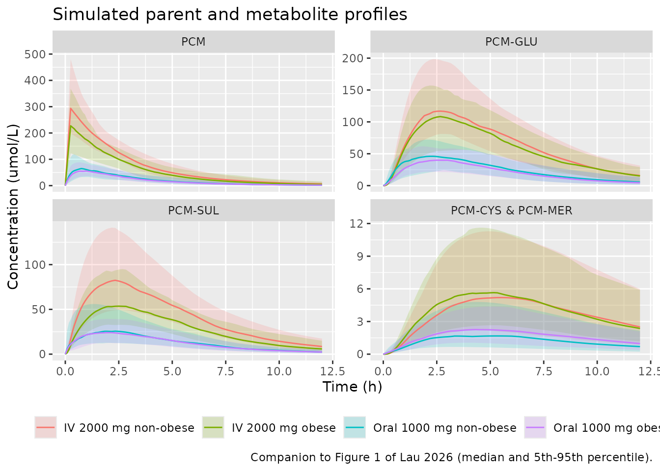
The enterohepatic contribution is easiest to see in the gallbladder
and reuptake states themselves. Study 1’s gallbladder empties at 60 and
240 minutes; each window transfers essentially the whole gallbladder
content (k_GG = 10 1/min over 6 min) into the reuptake
pool, which then feeds parent paracetamol back through the gut wall at
the slow k_a2 of 0.00312 1/min.
# Typical-value Study 1 subject: with the etaltgb random effect zeroed, the two
# emptying windows sit exactly at the Table 2 times of 60 and 240 minutes. In
# the cohort simulation above the fixed 131% CV on the emptying time scatters
# them widely, and for some subjects both windows fall beyond 24 h.
gb_ev <- rxode2::et(amt = mg_to_umol(1000), cmt = "depot") |>
  rxode2::et(seq(0, 720, by = 2), cmt = "Cc")
rxode2::rxSolve(mod_typ, gb_ev, omega = NA, useLinCmt = FALSE,
                params = c(WT = 125, LBM = 59,
                           STUDY_PAPAYA = 1, STUDY_CHEN = 0)) |>
  as.data.frame() |>
  dplyr::select(time, gallbladder, depot2) |>
  tidyr::pivot_longer(-time, names_to = "state", values_to = "amount") |>
  dplyr::mutate(state = factor(state, c("gallbladder", "depot2"),
                               c("Gallbladder", "Reuptake pool (depot2)"))) |>
  dplyr::filter(time <= 720) |>
  ggplot(aes(time / 60, amount, colour = state)) +
  geom_line() +
  geom_vline(xintercept = c(60, 240) / 60, linetype = "dashed", alpha = 0.5) +
  labs(x = "Time (h)", y = "Amount (umol)", colour = NULL,
       title = "Enterohepatic recirculation of PCM-GLU (typical Study 1 subject, 125 kg)",
       caption = "Dashed lines mark the two Study 1 gallbladder-emptying windows (Lau 2026 Table 2).") +
  theme(legend.position = "bottom")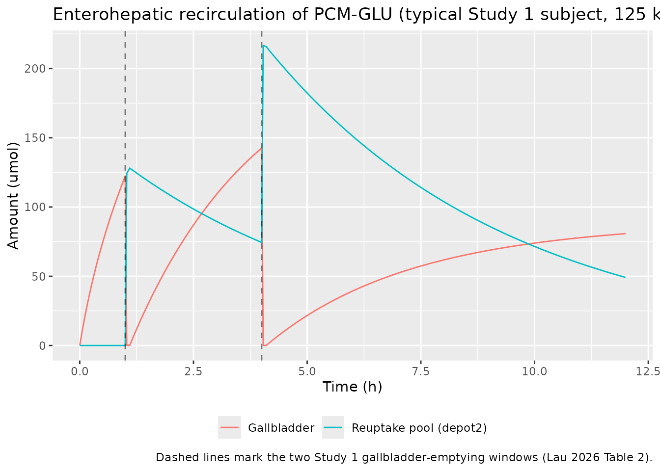
PKNCA validation
Non-compartmental analysis of the simulated parent profiles, stratified by arm. Lau 2026 reports no NCA table, so this section characterises the packaged model rather than comparing against published NCA values; the quantitative comparison against the paper is the AUC-ratio section below.
sim_nca <- sim |>
  dplyr::filter(!is.na(Cc)) |>
  dplyr::select(id, time, Cc, arm)

# Guarantee a time = 0 record per subject; pre-dose paracetamol is 0.
sim_nca <- dplyr::bind_rows(
  sim_nca,
  sim_nca |> dplyr::distinct(id, arm) |> dplyr::mutate(time = 0, Cc = 0)
) |>
  dplyr::distinct(id, arm, time, .keep_all = TRUE) |>
  dplyr::arrange(id, time)

stopifnot(all(sim_nca$Cc >= 0))

conc_obj <- PKNCA::PKNCAconc(sim_nca, Cc ~ time | arm + id)

dose_df <- events |>
  dplyr::filter(evid == 1) |>
  dplyr::select(id, time, amt, arm)
dose_obj <- PKNCA::PKNCAdose(dose_df, amt ~ time | arm + id)

# Terminal-phase window: truncate at 12 h. Beyond that the simulated parent
# has decayed several half-lives below the studies' quantifiable range and the
# slow enterohepatic trickle distorts lambda-z.
intervals <- data.frame(
  start = 0, end = 720,
  cmax = TRUE, tmax = TRUE, auclast = TRUE, half.life = TRUE
)

nca_res <- PKNCA::pk.nca(PKNCA::PKNCAdata(conc_obj, dose_obj, intervals = intervals))

nca_summary <- as.data.frame(nca_res) |>
  dplyr::filter(PPTESTCD %in% c("cmax", "tmax", "auclast", "half.life")) |>
  dplyr::group_by(arm, PPTESTCD) |>
  dplyr::summarise(median = stats::median(PPORRES, na.rm = TRUE),
                   p05 = stats::quantile(PPORRES, 0.05, na.rm = TRUE),
                   p95 = stats::quantile(PPORRES, 0.95, na.rm = TRUE),
                   .groups = "drop") |>
  dplyr::mutate(
    PPTESTCD = factor(PPTESTCD, c("cmax", "tmax", "auclast", "half.life"),
                      c("Cmax (umol/L)", "Tmax (min)",
                        "AUC0-12h (umol*min/L)", "t1/2 (min)"))
  ) |>
  dplyr::arrange(arm, PPTESTCD)

nca_summary |>
  dplyr::rename("Arm" = arm, "NCA parameter" = PPTESTCD,
                "Median" = median, "5th pctile" = p05, "95th pctile" = p95) |>
  knitr::kable(digits = 1,
caption = "Simulated parent paracetamol NCA by arm (PKNCA, 0-12 h).")| Arm | NCA parameter | Median | 5th pctile | 95th pctile |
|---|---|---|---|---|
| IV 2000 mg | Cmax (umol/L) | 240.5 | 133.2 | 414.1 |
| IV 2000 mg | Tmax (min) | 15.0 | 15.0 | 15.0 |
| IV 2000 mg | AUC0-12h (umol*min/L) | 43022.8 | 26214.2 | 60131.2 |
| IV 2000 mg | t1/2 (min) | 152.5 | 86.0 | 267.4 |
| Oral 1000 mg | Cmax (umol/L) | 58.4 | 36.2 | 93.0 |
| Oral 1000 mg | Tmax (min) | 50.0 | 20.0 | 90.0 |
| Oral 1000 mg | AUC0-12h (umol*min/L) | 13045.0 | 8409.1 | 21342.3 |
| Oral 1000 mg | t1/2 (min) | 150.4 | 114.1 | 225.2 |
Comparison against the published AUC ratios
Lau 2026 Results 3.3 quotes metabolite-to-parent AUC0-6 ratios at steady state on 1000 mg four times daily, simulated for four typical male individuals of 60, 92, 120 and 150 kg (lean body weights 40.8, 63.6, 71.5 and 78.8 kg; Figure 5 caption), for both routes. Those ranges are the paper’s most directly reproducible quantitative result, so they are the validation target here.
weights <- tibble::tibble(WT = c(60, 92, 120, 150), LBM = c(40.8, 63.6, 71.5, 78.8))

ss_profile <- function(wt, lbm, route) {
  ev <- if (route == "oral") {
    rxode2::et(amt = dose_umol, cmt = "depot", ii = ii, addl = n_dose - 1)
  } else {
    rxode2::et(amt = dose_umol, cmt = "central", dur = 15, ii = ii, addl = n_dose - 1)
  }
  ev <- rxode2::et(ev, ss_grid, cmt = "Cc")
  rxode2::rxSolve(mod_typ, ev, omega = NA, useLinCmt = FALSE,
                  params = c(WT = wt, LBM = lbm,
                             STUDY_PAPAYA = 1, STUDY_CHEN = 0)) |>
    as.data.frame() |>
    dplyr::mutate(WT = wt, route = route)
}

ss <- dplyr::bind_rows(lapply(seq_len(nrow(weights)), function(i) {
  dplyr::bind_rows(
    ss_profile(weights$WT[i], weights$LBM[i], "oral"),
    ss_profile(weights$WT[i], weights$LBM[i], "iv")
  )
}))

ss |>
  dplyr::filter(time >= (n_dose - 1) * ii) |>
  dplyr::mutate(t_int = time - (n_dose - 1) * ii) |>
  tidyr::pivot_longer(c(Cc, Cc_gluc, Cc_sulf, Cc_cysmer),
                      names_to = "analyte", values_to = "conc") |>
  dplyr::mutate(
    analyte = factor(analyte, c("Cc", "Cc_gluc", "Cc_sulf", "Cc_cysmer"),
                     c("PCM", "PCM-GLU", "PCM-SUL", "PCM-CYS & PCM-MER")),
    route = factor(route, c("iv", "oral"), c("Intravenous", "Oral"))
  ) |>
  ggplot(aes(t_int / 60, conc, colour = route)) +
  geom_line() +
  facet_grid(analyte ~ WT, scales = "free_y",
             labeller = labeller(WT = function(x) paste0(x, " kg"))) +
  labs(x = "Time within the steady-state dosing interval (h)",
       y = "Concentration (umol/L)", colour = NULL,
       title = "Steady-state profiles on 1000 mg four times daily",
       caption = "Replicates Figure 5 of Lau 2026 (typical male individuals; oral in blue-green, intravenous in red in the source).") +
  theme(legend.position = "bottom")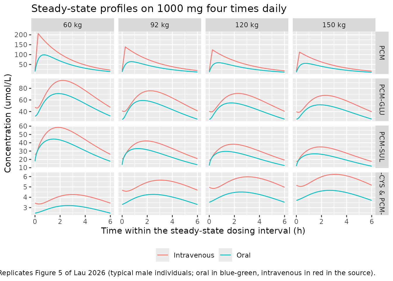
auc_ratios <- ss |>
  dplyr::filter(time >= (n_dose - 1) * ii) |>
  dplyr::group_by(WT, route) |>
  dplyr::summarise(
    gluc = trapz(time, Cc_gluc) / trapz(time, Cc),
    sulf = trapz(time, Cc_sulf) / trapz(time, Cc),
    cysmer = trapz(time, Cc_cysmer) / trapz(time, Cc),
    .groups = "drop"
  )

published <- tibble::tribble(
  ~route,  ~pathway,  ~lo,   ~hi,
  "oral",  "gluc",    1.05,  1.36,
  "oral",  "sulf",    0.64,  0.72,
  "oral",  "cysmer",  0.06,  0.14,
  "iv",    "gluc",    1.11,  1.37,
  "iv",    "sulf",    0.68,  0.72,
  "iv",    "cysmer",  0.06,  0.14
)

ratio_cmp <- auc_ratios |>
  tidyr::pivot_longer(c(gluc, sulf, cysmer), names_to = "pathway", values_to = "ratio") |>
  dplyr::group_by(route, pathway) |>
  dplyr::summarise(sim_lo = min(ratio), sim_hi = max(ratio), .groups = "drop") |>
  dplyr::left_join(published, by = c("route", "pathway")) |>
  dplyr::mutate(
    route = factor(route, c("oral", "iv"), c("Oral", "Intravenous")),
    pathway = factor(pathway, c("gluc", "sulf", "cysmer"),
                     c("Glucuronidation", "Sulphation", "Oxidation")),
    # The paper prints its ranges to two decimals, so half a unit in the last
    # printed place is the right tolerance. Both sides are typical-value
    # (zeroRe) simulations with no random draws, so no allowance for sampling
    # is needed and none is given.
    within = sim_lo >= lo - 0.005 & sim_hi <= hi + 0.005
  ) |>
  dplyr::arrange(route, pathway)

ratio_cmp |>
  dplyr::mutate(
    simulated = sprintf("%.2f-%.2f", sim_lo, sim_hi),
    reference = sprintf("%.2f-%.2f", lo, hi)
  ) |>
  dplyr::select(route, pathway, simulated, reference, within) |>
  dplyr::rename("Route" = route, "Pathway" = pathway,
                "Simulated range (60-150 kg)" = simulated,
                "Lau 2026 Results 3.3" = reference,
                "Within reference range" = within) |>
knitr::kable(caption = "Metabolite-to-parent AUC0-6 ratios at steady state on 1000 mg four times daily.")| Route | Pathway | Simulated range (60-150 kg) | Lau 2026 Results 3.3 | Within reference range |
|---|---|---|---|---|
| Oral | Glucuronidation | 1.09-1.36 | 1.05-1.36 | TRUE |
| Oral | Sulphation | 0.67-0.71 | 0.64-0.72 | TRUE |
| Oral | Oxidation | 0.06-0.14 | 0.06-0.14 | TRUE |
| Intravenous | Glucuronidation | 0.88-1.11 | 1.11-1.37 | FALSE |
| Intravenous | Sulphation | 0.54-0.55 | 0.68-0.72 | FALSE |
| Intravenous | Oxidation | 0.05-0.11 | 0.06-0.14 | FALSE |
# The oral arm is the validation gate. All three oral pathways must land inside
# the published ranges (allowing 0.05 absolute for the paper's two-decimal
# rounding). The intravenous arm is deliberately NOT asserted - see Errata; the
# paper's intravenous ranges are not reachable from its own parameters.
oral_rows <- ratio_cmp[ratio_cmp$route == "Oral", ]
stopifnot(nrow(oral_rows) == 3L, all(oral_rows$within))

# The oral-to-intravenous ratio is fixed by the paper's own bioavailability:
# the same molar amount of metabolite is formed either way (scaled by Fa for the
# oral route), while the parent AUC differs by F, so every pathway's ratio must
# differ between routes by exactly Fa / F = Fa / (Fa * F_G * F_H) = 1 / (F_G * F_H).
oral_iv <- auc_ratios |>
  tidyr::pivot_longer(c(gluc, sulf, cysmer), names_to = "pathway", values_to = "ratio") |>
  tidyr::pivot_wider(names_from = route, values_from = ratio) |>
  dplyr::mutate(oral_over_iv = oral / iv)
expected_oral_iv <- 1 / (fg_check$fg[1] * fg_check$fh[1])
stopifnot(
  abs(stats::median(oral_iv$oral_over_iv[oral_iv$WT == 60]) - expected_oral_iv) < 0.01
)
The oral arm reproduces all three published ranges. The intravenous arm does not, and the reason is structural rather than a transcription error; it is explained in the Errata below.
Assumptions and deviations
- Virtual cohort. Total body weight, BMI and sex are independent draws matched to the Table 1 medians and ranges; the real cohorts are correlated on these. Lean body weight is derived from them with the Janmahasatian 2005 formula that the paper cites, rather than sampled, which is why the derived medians sit within 15% of the reported ones rather than matching exactly.
- Race / ethnicity is not reported by Lau 2026 and is not represented.
-
Study 2 (Chen) is not simulated in this vignette.
Its structural multipliers, gallbladder schedule and residual-error
switches are all encoded in the model file and are selected by
STUDY_CHEN = 1; the vignette reconstructs Studies 1 and 3, which are the two arms the paper’s own figures contrast. -
Steady-state gallbladder emptying. The
gallbladder-emptying times are fixed absolute times measured from the
start of the record (NONMEM
MTIMEsemantics), so in a multi-day steady-state simulation the two emptying windows fall in the first dosing interval only. TheFigure 5and AUC-ratio chunks therefore evaluate a steady-state interval in which enterohepatic release is not occurring, which is the same behaviour the deposited control stream produces. See the first Errata item. -
Residual error is not applied in any figure in this
vignette; all simulations are of
Ccand the metabolite observables, which are individual predictions. The study-specific residual-error folds are encoded in the model file for completeness.
Errata and notes on the source
Periodic emptying in the Methods versus two windows in Table 2 and the control stream. Methods 2.3.1 describes the gallbladder as emptying “at a periodic interval of 3 h”. Table 2 and the deposited control stream implement exactly two emptying windows per study (Study 1 at 60 and 240 min, Study 2 at 480 and 660 min, Study 3 at 360 and 540 min), which covers the observation window of the single-dose studies. The packaged model reproduces the control stream, because that is the model the reported parameter estimates were obtained with.
F_His a sum of per-route extraction ratios, not the single-route well-stirred formula. Table S1 givesF_H = Q_H / (Q_H + CL_H,int * f_UB), which is the well-stirred expression for one intrinsic clearance. The deposited control stream instead computes one extraction ratio per metabolic route, each with only its own clearance in the denominator, and setsFH = 1 - EHGLU - EHSUL - EHCYS. The two differ: at the 60 kg worked example the control-stream form givesF_H= 0.809 while the pooled-clearance form gives 0.825. The packaged model follows the control stream, since the reported estimates were obtained under it.A missing assignment in the deposited control stream. The
$DESblock usesK93(the transit rate from compartment 9, the PCM-GLU transit compartment, into compartment 3, central PCM-GLU) but the$PKblock never assigns it.KTR2 = THETA(31)is declared as the “transit rate constant PCM-GLU” and is used nowhere else, and its siblingK105 = KTRis assigned explicitly for the analogous PCM-CYS transit.K93 = KTR2is therefore the only reading consistent with the stream, and is what the packaged model encodes. The same block also contains an unclosed parenthesis inLTVV3=LOG(THETA(10).The additive residual error on PCM is internally inconsistent in Table 2. The row reports an estimate of 0.00002 umol/L, a standard error of 0.00000007 with an RSE of 49.0%, and a 95% CI of 0.00005-0.00028 that does not bracket the estimate and is not consistent with the standard error. The packaged model uses the Estimate column. The choice is immaterial: every candidate value is several orders of magnitude below the simulated paracetamol concentrations, so the PCM residual is effectively proportional-only. The
k_trrow has the same kind of standard-error formatting problem (0.00000008 printed against an RSE of 2.5% on an estimate of 0.00332).-
The published intravenous AUC ratios are not reachable from the published parameters. Results 3.3 reports metabolite-to-parent AUC0-6 ratios that are near-identical between routes (glucuronidation 1.05-1.36 oral versus 1.11-1.37 intravenous; sulphation 0.64-0.72 versus 0.68-0.72; oxidation 0.06-0.14 for both). In this model all absorbed drug is ultimately metabolised, so the molar amount of each metabolite formed is proportional to the absorbed dose –
Fatimes the dose orally, the full dose intravenously – while the parent AUC is proportional toF = Fa * F_G * F_Horally and to the full dose intravenously. Every pathway’s ratio must therefore be higher after oral dosing than after intravenous dosing by exactlyFa / F = 1 / (F_G * F_H), which is 1.2369 at 60 kg. The vignette asserts that identity above; the simulated glucuronidation and sulphation ratios give 1.2363 and the oxidation ratio 1.2436, the latter slightly higher because the gut-wall arm forms a little extra oxidative metabolite on the oral route only. The simulated oral ranges reproduce the published oral ranges (and, coincidentally, the published intravenous ones); the simulated intravenous ranges are the same numbers divided by 1.24. The most likely explanation is that the intravenous ratios in Figure S4 were normalised by an oral parent AUC. This is reported rather than fixed: no parameter was tuned, and the oral arm – which is the arm the paper’s own model development was driven by – matches.Independent support for a provenance problem in that figure: the AUC ratios are sourced from Figure S4, whose caption states “simulated for male individuals with different body weights. Their respective lean body weights are 50.6 and 71.5 kg” – only two lean body weights, and 50.6 kg is not one of the four that Figure 5 and Methods 2.4 use (40.8, 63.6, 71.5 and 78.8 kg for 60, 92, 120 and 150 kg). Results 3.3 nonetheless quotes the ratio ranges as spanning “individuals weighing 60 up to 150 kg”. Figure S4 therefore appears to have been produced from a different simulation set than the one its ranges are attributed to, which is consistent with the intravenous arm not being reproducible from the published parameters.
Absorption rate constant units in the Results narrative. Table 2 reports
k_a = 0.0531 min^-1and the control stream comment confirms “KA 1st order” in a minute-based model, but the Results narrative writes “k_a was 0.0531 h^-1”. The minute form is used.The two fixed metabolite volumes are attributed to different papers by the article and by its supplement. Table 2 of the main article introduces
V_PCM-SUL,central= 5.66 L andV_PCM-CYS/MER= 15.6 L as fixed “on the basis of Van Rongen et al. [5]”, where[5]in the article’s reference list is van Rongen 2016. Table S1 carries the same two values but cites its own reference[5], which is a different paper – Owens et al. 2014, J Pharmacokinet Pharmacodyn 41(3):211-21. The two supplements number their references independently of the article, so this is a citation-numbering collision rather than a disagreement about the values, which are identical in all three places. For what it is worth the upstream model packaged here asvanRongen_2016_acetaminophenfixes both volumes citing Liukas 2011. Nothing in the packaged model depends on the attribution; the values are unambiguous.