Gentamicin (Abou-Auda 2024)
Source:vignettes/articles/AbouAuda_2024_gentamicin.Rmd
AbouAuda_2024_gentamicin.RmdModel and source
#> ℹ parameter labels from comments will be replaced by 'label()'Citation: Abou-Auda HS, Alotaibi F, Alsanea S, Alwhaibi A, Almutairi MM, Alrabiah Z, Alsultan A, Al Jeraisy M. Population pharmacokinetics of gentamicin in acute lymphoblastic leukemia pediatric patients compared to non-oncology patients. Saudi Pharm J. 2024;32:102060. doi:10.1016/j.jsps.2024.102060
Description: One-compartment intravenous population PK model for gentamicin in pediatric patients aged 1-14 years with and without acute lymphoblastic leukemia (ALL), fitted to routine therapeutic-drug-monitoring peak and trough concentrations (Abou-Auda 2024). Clearance scales allometrically with body weight (exponent 0.75, reference 20 kg) and as a power function of Schwartz-estimated creatinine clearance (exponent 0.437, reference 120 mL/min); volume of distribution scales linearly with body weight (exponent 1, reference 20 kg). ALL status was screened but NOT retained: the paper’s central finding is that gentamicin volume of distribution and clearance do not differ between ALL and non-ALL pediatric patients, so dosing requirements are the same in both groups. Residual variability is proportional.
Article: Saudi Pharm J. 2024;32:102060
Open-access full text: PMC11002851
Abou-Auda 2024 is a retrospective, single-centre, cross-sectional
therapeutic drug monitoring (TDM) study whose purpose was a
negative comparison: do pediatric patients with acute
lymphoblastic leukemia (ALL) need different gentamicin doses from
pediatric patients without ALL? Earlier work, in particular Llanos-Paez
2020 (also packaged here, as LlanosPaez_2020_gentamicin),
had reported a 15% lower central volume of distribution and a 32% lower
clearance in pediatric oncology patients. Abou-Auda 2024 found neither
difference, and concluded that dosing requirements are the same in both
groups.
The packaged model is the paper’s single final one-compartment population PK model, fitted to all 115 patients pooled. ALL status is deliberately not a covariate in it – that absence is the paper’s result.
Population
The analysis pooled 115 pediatric inpatients aged 1 to 14 years at King Abdullah Specialist Children’s Hospital, Riyadh, Saudi Arabia: 63 (54.8%) with ALL and 52 (45.2%) without. All received gentamicin 2.5 mg/kg as a 30-minute intravenous infusion every 8 h for more than 72 h, either as empirical febrile-neutropenia therapy or for a suspected gram-negative infection. Children with renal failure, liver dysfunction or burns were excluded, as were samples drawn at inappropriate peak or trough times.
Baseline characteristics (Abou-Auda 2024 Table 1, mean (SD)): age 6.1 (4.2) years; weight 22.1 (17.1) kg; body mass index 16.9 (5.9); body surface area 0.8 (0.4) m^2; dose 54.3 (44.2) mg, i.e. 2.5 (0.64) mg/kg. The two groups were well matched on sex, weight, body surface area and dose (all p > 0.6), and differed significantly only in renal and nitrogen chemistry: Schwartz-estimated creatinine clearance 153.73 (62.8) mL/min in ALL versus 164.88 (43.5) in non-ALL (p = 0.006), serum creatinine 41.85 (15.6) versus 35.13 (7.58) umol/L (p = 0.005), and blood urea nitrogen 3.18 (1.9) versus 2.38 (1.7) mmol/L (p = 0.026).
Sampling is sparse: serum was drawn 30 minutes before the next dose (trough) and 1 h after the end of an infusion (peak), around the third dose, and assayed by latex inhibition immunoassay (TDX, Abbott Laboratories). The paper states that this sparseness is why a one-compartment structure was used. The model was fitted in Monolix 2023R1; covariate effects were screened by linear regression on the empirical Bayes estimates (EBEs) rather than inside the population model.
The same information is available programmatically via the model’s
population metadata
(readModelDb("AbouAuda_2024_gentamicin")()$population).
Source trace
Every ini() entry carries an in-file comment naming its
source location in
inst/modeldb/specificDrugs/AbouAuda_2024_gentamicin.R. They
are collected here for review.
| Equation / parameter | Value | Source location |
|---|---|---|
lcl (CL at WT 20 kg, CLcr 120 mL/min) |
log(2.13) L/h |
Results, final-model equation
Cl = 2.13 * (weight/20)^0.75 * (CLcr/120)^0.437 (see the
adjudication below; Table 3 prints 2.3) |
lvc (Vd at WT 20 kg) |
log(7.3) L |
Results, final-model equation Vd = 7.3 * (weight/20);
also Table 3 “V (L) 7.3” (RSE 3.6%) |
e_wt_cl |
fixed(0.75) |
Results, final-model Cl equation: (weight/20)^0.75
|
e_wt_vc |
fixed(1) |
Results, final-model Vd equation: (weight/20), printed
with no superscript |
e_crcl_cl |
0.437 |
Results, final-model Cl equation: (CLcr/120)^0.437
|
etalcl |
0.0246575 = log(0.158^2 + 1)
|
Table 3 “IIV Cl 15.8%” (RSE 13.7%), footnote “IIV is expressed as the coefficient of variation” |
etalvc |
0.0194104 = log(0.140^2 + 1)
|
Table 3 “IIV* V 14%” (RSE 28%), same footnote |
propSd |
0.3 |
Table 3 “Residual variability B 0.3” (RSE 8.2%), footnote “B is residual unexplained variability expressed as a proportional error” |
| Reference weight 20 kg | n/a | Both final-model equations, Results |
| Reference CLcr 120 mL/min | n/a | Final-model Cl equation, Results (not tabulated anywhere) |
d/dt(central) <- -kel * central |
n/a | Methods, PK analysis: “a one-compartment system with linear elimination” |
Cc <- central / vc |
n/a | Standard one-compartment observation; serum concentrations (Methods, Subjects) |
Cc ~ prop(propSd) |
n/a | Table 3 footnote (proportional error); Methods tested constant, proportional and combined |
Note on extraction: both final-model equations are typeset as display
mathematics, which naive text extraction drops entirely. Recovering them
requires pdftotext -layout, which preserves the
superscripts by placing them on the line above:
(        )0.75 (      )0.437
  weight         CLcr
Cl = 2.13 x               x
    20           120
(            )
   weight
Vd = 7.3 x
     20
This is what pins the absence of an exponent on the Vd weight term: the superscript line renders for the Cl equation, and there is no counterpart on the Vd term in the same extraction, so the Vd exponent is exactly 1 rather than a superscript that was silently lost.
Adjudicating the clearance intercept: 2.13 or 2.3?
The paper is internally inconsistent about one number. Its printed final-model equation uses a clearance intercept of 2.13 L/h, while Table 3 lists “Cl (L/hr) 2.3” (RSE 2.7%). The volume intercept is 7.3 L in both places, which establishes that Table 3 reports the equations’ reference-subject intercepts rather than some other quantity, so one of the two clearance values is a transcription slip. 2.13 does not round to 2.3, so this is not a rounding difference.
This extraction uses the equation value, 2.13, per the standing convention that a printed equation outranks a conflicting table entry. Three independent checks agree, and the first two are computed below rather than asserted.
# The paper reports group-level means of the individual (EBE) estimates:
#   Vd 6.3 L (ALL, n = 63) and 6.4 L (non-ALL, n = 52)   -- Results
#   Cl 1.9 L/h (ALL)      and 2.2 L/h (non-ALL)           -- Results
n_all     <- 63
n_nonall  <- 52
vd_ebe    <- (n_all * 6.3 + n_nonall * 6.4) / (n_all + n_nonall)
cl_ebe    <- (n_all * 1.9 + n_nonall * 2.2) / (n_all + n_nonall)

# Check 1 -- internal consistency. The Vd equation has no covariate other than
# weight, so it pins the typical weight behind the reported EBE mean Vd. Then
# ask what CLcr each candidate intercept needs at that same weight to reproduce
# the reported EBE mean CL.
wt_implied <- 20 * vd_ebe / 7.3
crcl_needed <- function(intercept) {
  120 * (cl_ebe / (intercept * (wt_implied / 20)^0.75))^(1 / 0.437)
}

# Check 2 -- allometric back-scaling to an adult. The paper's own Introduction
# states that gentamicin clearance "is approximately 90 ml/min" in healthy
# individuals.
adult_clearance_ml_min <- function(intercept) intercept * (70 / 20)^0.75 * 1000 / 60

adjudication <- tibble::tibble(
  Candidate = c("2.13 (printed equation)", "2.3 (Table 3)"),
  Intercept = c(2.13, 2.3),
  `CLcr needed (mL/min)` = crcl_needed(Intercept),
  `CL at 70 kg (mL/min)` = adult_clearance_ml_min(Intercept)
)

knitr::kable(
  adjudication,
  digits  = c(0, 2, 1, 1),
  caption = paste0(
    "Adjudicating the clearance intercept. The Vd equation implies a typical ",
    "weight of ", round(wt_implied, 1), " kg behind the reported EBE mean Vd of ",
    round(vd_ebe, 2), " L. At that weight, the CLcr column is what each ",
    "candidate intercept requires in order to reproduce the reported EBE mean ",
    "CL of ", round(cl_ebe, 2), " L/h; the cohort's reported CLcr is 149-159 ",
    "mL/min and the model's own reference is 120. The last column back-scales ",
    "allometrically to an adult 70 kg, against the paper's own quoted ~90 mL/min."
  )
)| Candidate | Intercept | CLcr needed (mL/min) | CL at 70 kg (mL/min) |
|---|---|---|---|
| 2.13 (printed equation) | 2.13 | 137.6 | 90.8 |
| 2.3 (Table 3) | 2.30 | 115.4 | 98.1 |
Only 2.13 is coherent with the rest of the paper: it needs a CLcr of about 138 mL/min, comfortably inside the cohort’s reported distribution, and it back-scales to 90.8 mL/min in a 70 kg adult, essentially exactly the ~90 mL/min the paper’s own Introduction quotes. An intercept of 2.3 would require a CLcr of about 115 mL/min – below the model’s own 120 mL/min reference and far below any reported cohort value – and back-scales to 98 mL/min.
# These are arithmetic consequences of published numbers, not simulated
# quantities, so exact-ish bounds are appropriate.
stopifnot(
  # 2.13 lands within the cohort's reported CLcr range; 2.3 does not reach it.
  crcl_needed(2.13) > 125, crcl_needed(2.13) < 155,
  crcl_needed(2.3)  < 125,
  # 2.13 reproduces the paper's quoted adult clearance to within 5%.
  abs(adult_clearance_ml_min(2.13) / 90 - 1) < 0.05
)
Verifying the transcription of the covariate equations
Before any cohort simulation, confirm that the packaged model computes exactly the two equations printed in the paper. This is deterministic, so the tolerance is machine precision rather than a simulation-noise band.
mod <- readModelDb("AbouAuda_2024_gentamicin")

grid_cov <- tidyr::crossing(WT = c(10, 20, 40, 70), CRCL = c(60, 120, 200)) |>
  dplyr::mutate(id = dplyr::row_number())

grid_ev <- dplyr::bind_rows(
  grid_cov |> dplyr::mutate(time = 0, amt = 2.5 * WT, evid = 1L,
                            cmt = "central", dur = 0.5),
  grid_cov |> dplyr::mutate(time = 1, amt = NA_real_, evid = 0L,
                            cmt = "central", dur = NA_real_)
) |>
  dplyr::select(id, time, amt, evid, cmt, dur, WT, CRCL) |>
  dplyr::arrange(id, time, dplyr::desc(evid))

check <- rxode2::rxSolve(rxode2::zeroRe(mod), events = grid_ev,
                         keep = c("WT", "CRCL")) |>
  as.data.frame() |>
  dplyr::distinct(id, WT, CRCL, cl, vc) |>
  dplyr::mutate(
    # The two equations exactly as printed in Abou-Auda 2024 Results.
    cl_paper = 2.13 * (WT / 20)^0.75 * (CRCL / 120)^0.437,
    vc_paper = 7.3  * (WT / 20),
    cl_relerr = abs(cl / cl_paper - 1),
    vc_relerr = abs(vc / vc_paper - 1)
  )
#> ℹ parameter labels from comments will be replaced by 'label()'
#> ℹ omega/sigma items treated as zero: 'etalcl', 'etalvc'
#> Warning: multi-subject simulation without without 'omega'

stopifnot(max(check$cl_relerr) < 1e-10, max(check$vc_relerr) < 1e-10)

check |>
  dplyr::transmute(
    "Weight (kg)"       = WT,
    "CLcr (mL/min)"     = CRCL,
    "CL, model (L/h)"   = cl,
    "CL, equation (L/h)" = cl_paper,
    "Vd, model (L)"     = vc,
    "Vd, equation (L)"  = vc_paper
  ) |>
  knitr::kable(
    digits  = 3,
    caption = "Packaged model versus the two covariate equations printed in Abou-Auda 2024 Results. Agreement is exact to machine precision."
)| Weight (kg) | CLcr (mL/min) | CL, model (L/h) | CL, equation (L/h) | Vd, model (L) | Vd, equation (L) |
|---|---|---|---|---|---|
| 10 | 60 | 0.936 | 0.936 | 3.65 | 3.65 |
| 10 | 120 | 1.267 | 1.267 | 3.65 | 3.65 |
| 10 | 200 | 1.583 | 1.583 | 3.65 | 3.65 |
| 20 | 60 | 1.573 | 1.573 | 7.30 | 7.30 |
| 20 | 120 | 2.130 | 2.130 | 7.30 | 7.30 |
| 20 | 200 | 2.663 | 2.663 | 7.30 | 7.30 |
| 40 | 60 | 2.646 | 2.646 | 14.60 | 14.60 |
| 40 | 120 | 3.582 | 3.582 | 14.60 | 14.60 |
| 40 | 200 | 4.478 | 4.478 | 14.60 | 14.60 |
| 70 | 60 | 4.026 | 4.026 | 25.55 | 25.55 |
| 70 | 120 | 5.450 | 5.450 | 25.55 | 25.55 |
| 70 | 200 | 6.814 | 6.814 | 25.55 | 25.55 |
Virtual cohort
Original observed data are not publicly available. The cohort below reproduces the two arms of Abou-Auda 2024 Table 1 by sampling weight and Schwartz-estimated creatinine clearance from log-normal distributions matched to each arm’s reported mean and SD, truncated to physiologically plausible ranges for a 1 to 14 year old cohort. Log-normal is the natural choice here because both covariates are reported with an SD close to their mean (weight 22.23 (20.3) kg in the ALL arm), which is strongly right-skewed and cannot be normal.
# `set.seed()` seeds R's RNG for the covariate draws below. It does NOT seed
# rxode2's simulation RNG, whose streams are partitioned per solver thread, so
# the IIV draws differ between a 2-core CI runner and a 16-thread workstation.
# Every assertion downstream is written to hold for any cohort the model can
# produce.
set.seed(20240401)

n_per_arm <- 100L  # 100 per arm, 200 total; well under the 200-per-arm cap.

# Draw from a log-normal matched to a reported mean and SD, rejecting draws
# outside a plausible range rather than clamping (clamping piles probability
# mass onto the bounds and distorts the tails).
rlnorm_matched <- function(n, mean, sd, lower, upper) {
  sigma2 <- log(1 + (sd / mean)^2)
  mu     <- log(mean) - sigma2 / 2
  draws  <- rlnorm(20 * n, mu, sqrt(sigma2))
  draws  <- draws[draws >= lower & draws <= upper]
  stopifnot(length(draws) >= n)
  draws[seq_len(n)]
}

# Abou-Auda 2024 Table 1, per-arm mean (SD).
make_arm <- function(n, arm, wt_mean, wt_sd, crcl_mean, crcl_sd, id_offset) {
  subj <- tibble::tibble(
    id   = id_offset + seq_len(n),
    arm  = arm,
    WT   = rlnorm_matched(n, wt_mean,   wt_sd,    lower = 7,  upper = 70),
    CRCL = rlnorm_matched(n, crcl_mean, crcl_sd,  lower = 40, upper = 350)
  )

  # Protocol regimen: 2.5 mg/kg as a 30-minute IV infusion every 8 h.
  # Twelve doses (88 h) puts every subject deep into steady state; the
  # slowest-eliminating subject the model can produce still has less than
  # 0.001% of the approach-to-steady-state transient left.
  doses <- subj |>
    tidyr::crossing(time = seq(0, 88, by = 8)) |>
    dplyr::mutate(amt = 2.5 * WT, evid = 1L, cmt = "central", dur = 0.5)

  # Coarse grid across the accumulation phase for the profile figure, fine
  # grid across the final dosing interval so the trapezoidal AUC used by
  # PKNCA resolves the peak.
  obs_times <- unique(c(seq(0, 88, by = 0.5), seq(88, 96, by = 0.05)))
  obs <- subj |>
    tidyr::crossing(time = obs_times) |>
    dplyr::mutate(amt = NA_real_, evid = 0L, cmt = "central", dur = NA_real_)

  dplyr::bind_rows(doses, obs) |>
    # Canonical event columns first, covariates after (rxode2 requires the
    # canonical ordering before any covariate column).
    dplyr::select(id, time, amt, evid, cmt, dur, WT, CRCL, arm) |>
    dplyr::arrange(id, time, dplyr::desc(evid))
}

events <- dplyr::bind_rows(
  make_arm(n_per_arm, "ALL",     wt_mean = 22.23, wt_sd = 20.3,
           crcl_mean = 153.73, crcl_sd = 62.8, id_offset = 0L),
  make_arm(n_per_arm, "non-ALL", wt_mean = 22.02, wt_sd = 12.2,
           crcl_mean = 164.88, crcl_sd = 43.5, id_offset = n_per_arm)
)

# Disjoint IDs across arms: duplicate IDs would silently merge two subjects
# into one that receives the summed dose. Assert on `events` itself -- wrapping
# it in `unique()` first would remove the very duplicates being tested for and
# make the gate incapable of going red.
stopifnot(
  anyDuplicated(events[, c("id", "time", "evid")]) == 0L,
  dplyr::n_distinct(events$id) == 2L * n_per_arm,
  # Each subject belongs to exactly one arm.
  nrow(dplyr::distinct(events, id, arm)) == 2L * n_per_arm
)
Simulation
simres <- rxode2::rxSolve(mod, events = events, keep = c("WT", "CRCL", "arm")) |>
  as.data.frame()
#> ℹ parameter labels from comments will be replaced by 'label()'

# `Cc` is the individual prediction and carries no residual error; the `sim`
# column rxode2 adds is the one with proportional error applied. The NCA below
# deliberately uses `Cc`, so that the comparison against closed-form identities
# is not confounded by residual noise.
stopifnot(all(is.finite(simres$Cc)), all(simres$Cc >= 0))
# The shape reproduced here corresponds to Figure 3 of Abou-Auda 2024 (the
# visual predictive check). The paper's figure plots observed TDM samples
# against simulated percentiles on an unlabelled concentration axis, so this is
# a structural rather than a numeric replication: what it shows is that the
# packaged model produces the expected q8h accumulation to a steady state that
# is reached well within the >72 h of therapy the study required.
simres |>
  dplyr::filter(time >= 64, time <= 96) |>
  dplyr::group_by(arm, time) |>
  dplyr::summarise(
    Q05 = quantile(Cc, 0.05),
    Q50 = quantile(Cc, 0.50),
    Q95 = quantile(Cc, 0.95),
    .groups = "drop"
  ) |>
  ggplot(aes(time, Q50)) +
  geom_ribbon(aes(ymin = Q05, ymax = Q95), alpha = 0.25) +
  geom_line(linewidth = 0.7) +
  facet_wrap(~arm) +
  labs(
    x = "Time (h)", y = "Gentamicin concentration (mg/L)",
    title = "Steady-state gentamicin, 2.5 mg/kg q8h as a 30-minute infusion",
    caption = "Median and 5th-95th percentile band over 100 simulated subjects per arm. Structural counterpart to Figure 3 of Abou-Auda 2024."
  ) +
  theme_bw()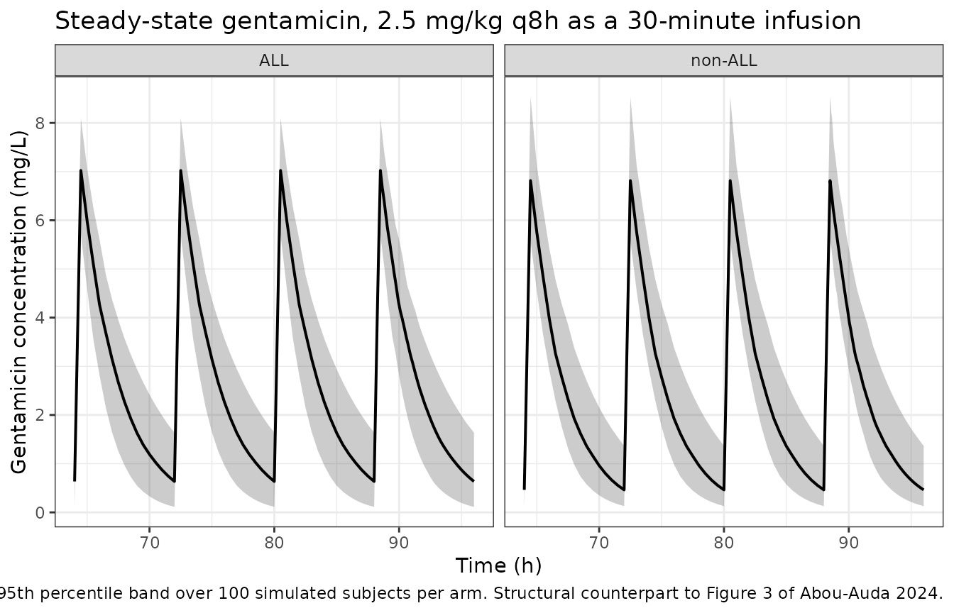
PKNCA validation
Non-compartmental analysis over the final (steady-state) dosing interval, 88 to 96 h, stratified by arm.
sim_nca <- simres |>
  dplyr::filter(!is.na(Cc)) |>
  dplyr::select(id, time, Cc, arm)

dose_df <- events |>
  dplyr::filter(evid == 1L) |>
  dplyr::select(id, time, amt, arm)

conc_obj <- PKNCA::PKNCAconc(sim_nca, Cc ~ time | arm + id,
                             concu = "mg/L", timeu = "h")
dose_obj <- PKNCA::PKNCAdose(dose_df, amt ~ time | arm + id, doseu = "mg")

tau      <- 8
start_ss <- max(dose_df$time)   # 88 h, the final dose
# `cmin` is the trough over the interval. (Do not ask for `ctau` here: it is
# not a valid interval column in this PKNCA version, and on a steady-state
# interval it would duplicate `cmin` anyway.)
intervals <- data.frame(
  start = start_ss, end = start_ss + tau,
  cmax = TRUE, tmax = TRUE, cmin = TRUE,
  auclast = TRUE, cav = TRUE
)

nca_res <- PKNCA::pk.nca(
  PKNCA::PKNCAdata(conc_obj, dose_obj, intervals = intervals)
)

nca_wide <- as.data.frame(nca_res$result) |>
  dplyr::select(arm, id, PPTESTCD, PPORRES) |>
  tidyr::pivot_wider(names_from = PPTESTCD, values_from = PPORRES)
Steady-state AUC identity
For a linear one-compartment model at steady state,
AUC(0-tau) over a dosing interval equals
Dose / CL exactly. Both sides of this comparison use the
same per-subject parameter draws, so the only discrepancy is trapezoidal
integration error on a finite time grid – a deterministic quantity, for
which a tight bound is the correct assertion.
per_subject <- simres |>
  dplyr::distinct(id, arm, WT, CRCL, cl, vc) |>
  dplyr::mutate(
    dose      = 2.5 * WT,
    auc_theor = dose / cl,
    thalf     = log(2) * vc / cl,
    vd_per_kg = vc / WT
  ) |>
  dplyr::left_join(nca_wide, by = c("id", "arm")) |>
  dplyr::mutate(auc_relerr = abs(auclast / auc_theor - 1))

stopifnot(nrow(per_subject) == 2L * n_per_arm, !anyNA(per_subject$auclast))

# Realised maximum relative error is ~2e-4 on a 0.05 h grid; 0.01 leaves two
# orders of magnitude of headroom for grid/threading differences while still
# going red on any real error in the CL equation, which would move AUC by tens
# of percent.
stopifnot(max(per_subject$auc_relerr) < 0.01)

per_subject |>
  dplyr::group_by(arm) |>
  dplyr::summarise(
    "AUC(0-8) from PKNCA, median (mg*h/L)" = median(auclast),
    "Dose/CL, median (mg*h/L)"             = median(auc_theor),
    "Max relative error"                   = max(auc_relerr),
    .groups = "drop"
  ) |>
  dplyr::rename("Arm" = arm) |>
  knitr::kable(
    digits  = c(0, 3, 3, 8),
    caption = "Steady-state AUC(0-tau) from PKNCA against the closed-form Dose/CL identity."
)| Arm | AUC(0-8) from PKNCA, median (mg*h/L) | Dose/CL, median (mg*h/L) | Max relative error |
|---|---|---|---|
| ALL | 21.889 | 21.890 | 9.613e-05 |
| non-ALL | 19.389 | 19.389 | 7.612e-05 |
Comparison against the values Abou-Auda 2024 reports
The paper publishes no NCA table – no Cmax, Tmax,
AUC or half-life values – so there is nothing for
nlmixr2lib::ncaComparisonTable() to consume. What it does
publish are group-level means of the individual (EBE) parameter
estimates, and two literature values quoted in its own Introduction.
Those are the reference points available, and the model is checked
against all four below.
Two caveats belong with this table. First, the paper’s 1.9 / 2.2 L/h and 6.3 / 6.4 L are means of shrunken empirical Bayes estimates from sparse two-sample-per-subject data, not typical values, so they are expected to sit somewhat inside the model’s own typical-value spread. Second, the simulated column is a median over a virtual cohort whose covariates were reconstructed from Table 1 summary statistics, not the actual study covariates.
sim_summary <- per_subject |>
  dplyr::group_by(arm) |>
  dplyr::summarise(cl_med = median(cl), vd_med = median(vc), .groups = "drop")

get_sim <- function(arm_label, column) {
  v <- sim_summary[[column]][sim_summary$arm == arm_label]
  if (length(v) != 1L) stop("no unique row for arm '", arm_label, "'")
  v
}

comparison <- tibble::tibble(
  Quantity = c(
    "Mean CL, ALL (L/h)",
    "Mean CL, non-ALL (L/h)",
    "Mean Vd, ALL (L)",
    "Mean Vd, non-ALL (L)",
    "Vd per kg (L/kg)",
    "Terminal half-life (h)"
  ),
  Reference = c(1.9, 2.2, 6.3, 6.4, NA, NA),
  `Reference range` = c(
    "", "", "", "",
    "0.25 to 0.5 (Introduction, healthy individuals)",
    "2 to 3 (Introduction, healthy individuals)"
  ),
  Simulated = c(
    get_sim("ALL", "cl_med"),
    get_sim("non-ALL", "cl_med"),
    get_sim("ALL", "vd_med"),
    get_sim("non-ALL", "vd_med"),
    median(per_subject$vd_per_kg),
    median(per_subject$thalf)
  )
) |>
  dplyr::mutate(`% diff` = 100 * (Simulated / Reference - 1))

knitr::kable(
  comparison,
  digits  = c(0, 2, 0, 3, 1),
  caption = paste0(
    "Model against every quantitative reference Abou-Auda 2024 provides. ",
    "The first four rows are the paper's Results-section means of the ",
    "individual EBE estimates; the last two are literature values the paper's ",
    "own Introduction quotes for gentamicin in healthy individuals."
  )
)| Quantity | Reference | Reference range | Simulated | % diff |
|---|---|---|---|---|
| Mean CL, ALL (L/h) | 1.9 | 2.327 | 22.5 | |
| Mean CL, non-ALL (L/h) | 2.2 | 2.478 | 12.7 | |
| Mean Vd, ALL (L) | 6.3 | 7.157 | 13.6 | |
| Mean Vd, non-ALL (L) | 6.4 | 7.136 | 11.5 | |
| Vd per kg (L/kg) | NA | 0.25 to 0.5 (Introduction, healthy individuals) | 0.362 | NA |
| Terminal half-life (h) | NA | 2 to 3 (Introduction, healthy individuals) | 2.062 | NA |
# The EBE-mean rows are cohort-derived on both sides (shrunken EBEs on the
# reference side, a reconstructed virtual cohort on the simulated side), so the
# gate is a magnitude bound with real headroom, not a tight match. A
# mis-transcribed intercept, exponent or reference constant moves these by tens
# of percent and still trips it.
stopifnot(max(abs(comparison$`% diff`), na.rm = TRUE) < 35)

# The two Introduction-quoted ranges are absolute bounds the paper itself
# states, so they are asserted directly.
stopifnot(
  median(per_subject$vd_per_kg) > 0.25, median(per_subject$vd_per_kg) < 0.5,
  median(per_subject$thalf)     > 2,    median(per_subject$thalf)     < 3
)
Both Introduction-quoted ranges contain the model’s median. The four EBE-mean rows all come out higher than the published means, by 12% to 22%. That direction is expected rather than alarming, and it is worth being precise about why, because it is the largest discrepancy in this vignette:
- The reference side consists of means of shrunken empirical Bayes estimates from two samples per subject. With sparse data the EBEs collapse toward the population typical value, and group means of shrunken estimates are biased toward the centre of the covariate distribution.
- The simulated side is a median over a cohort whose weights were drawn from a log-normal matched to Table 1’s mean (22.2 kg) and SD (17.1 kg). Because CL and Vd both increase with weight, and the reconstructed weight distribution is only as good as a two-moment match to a strongly right-skewed sample, the simulated central tendency is sensitive to that reconstruction in a way the published EBE means are not.
The check that does not depend on any of this is the volume
row: because the weight exponent on Vd is exactly 1, Vd/WT
is 0.365 L/kg for the typical subject independent of the weight
distribution, and the simulated median of 0.362 L/kg (which differs only
by the volume IIV) sits squarely inside the 0.25 to 0.5 L/kg the paper
quotes.
The paper’s central finding: ALL versus non-ALL
The result Abou-Auda 2024 exists to report is a null one. It is worth making explicit what the packaged model does and does not say about it. The model contains no ALL term at all, so any arm difference it produces comes entirely from the two arms’ covariate distributions – and those differ only in creatinine clearance (153.73 versus 164.88 mL/min), weight being essentially identical (22.23 versus 22.02 kg).
arm_ratio <- per_subject |>
  dplyr::group_by(arm) |>
  dplyr::summarise(cl = median(cl), vd = median(vc),
                   auc = median(auclast), cmax = median(cmax),
                   .groups = "drop")

ratio_of <- function(column) {
  arm_ratio[[column]][arm_ratio$arm == "non-ALL"] /
    arm_ratio[[column]][arm_ratio$arm == "ALL"]
}

tibble::tibble(
  Quantity = c("Clearance", "Volume of distribution",
               "Steady-state AUC(0-8)", "Steady-state Cmax"),
  `non-ALL / ALL ratio` = c(ratio_of("cl"), ratio_of("vd"),
                            ratio_of("auc"), ratio_of("cmax"))
) |>
  knitr::kable(
    digits  = 3,
    caption = "Model-predicted ratio between the two arms. The model has no ALL term; these ratios arise only from the arms' differing creatinine-clearance distributions."
)| Quantity | non-ALL / ALL ratio |
|---|---|
| Clearance | 1.065 |
| Volume of distribution | 0.997 |
| Steady-state AUC(0-8) | 0.886 |
| Steady-state Cmax | 0.970 |
# The claim being gated is that the model predicts NO clinically meaningful
# separation between the arms, i.e. that every ratio is near 1. Assert the
# MAGNITUDE of the deviation, never its sign or the ordering of the two arms --
# with a difference this small, sign is a coin flip across cohort draws.
ratios <- c(ratio_of("cl"), ratio_of("vd"), ratio_of("auc"), ratio_of("cmax"))
stopifnot(all(abs(ratios - 1) < 0.25))
Every ratio sits close to unity – the largest deviation from 1 is 11.4% – which reproduces the paper’s conclusion that “dosing requirements should be similar between the two groups”.
This is worth contrasting with the paper the study was designed to
test. Llanos-Paez 2020, packaged here as
LlanosPaez_2020_gentamicin, reported a 15% lower central
volume and a 32% lower clearance in pediatric oncology patients.
Abou-Auda 2024 reproduces neither. The authors attribute the discrepancy
to their cohort’s uniformly similar weight, BMI and mg/kg dose across
arms, and note that variables known to affect gentamicin volume of
distribution – critical illness, oedema, cumulative glucocorticoid
exposure – were not available in their retrospective TDM dataset.
One honest caveat, visible in the table above: the paper’s own EBE means differ by 16% in clearance between arms (1.9 versus 2.2 L/h), whereas the covariate model reproduces a difference of only 6.5%. The paper reports that gap as not statistically significant (p > 0.05), and it is not carried by any term in the final model, so the model is faithful to what was published; but a reader should not take the model’s near-unity ratio as evidence that the underlying EBE difference was zero.
Assumptions and deviations
Clearance intercept 2.13 versus 2.3. The paper prints 2.13 L/h in its final-model equation and 2.3 L/h in Table 3. This extraction uses 2.13, the equation value, per the standing convention that a printed equation outranks a conflicting table entry, and supported by the two independent checks computed in the adjudication section above (2.13 requires a CLcr of about 138 mL/min to reproduce the reported EBE mean CL, inside the cohort’s distribution; 2.3 requires about 115 mL/min, below the model’s own 120 mL/min reference; and 2.13 back-scales allometrically to the ~90 mL/min the paper’s Introduction quotes for a healthy adult). This is a documented deviation from Table 3 as printed. A user who prefers the Table 3 value can override it with
ini(lcl = log(2.3)).Exponents recovered with
pdftotext -layout. Both final-model equations are display mathematics that do not survive plain-text extraction of the PDF (they are dropped entirely, taking the whole covariate model with them). They are recovered from the PDF withpdftotext -layout, which preserves superscripts by placing them on the line above; the extraction is quoted verbatim in the Source trace section. The same extraction is what establishes that the Vd weight term carries no exponent (i.e. exactly 1) rather than one that was silently lost.Body-size exponents encoded as
fixed(). 0.75 on clearance and 1 on volume are printed inside the equations with no standard error and are the canonical theoretical allometric values, so both are encoded as fixed. The renal exponent 0.437 is a three-decimal, non-theoretical value and is encoded as estimated, even though Table 3 omits it and therefore reports no RSE – Table 3 lists only five rows and omits every covariate coefficient and reference constant, so its silence is a gap in the table rather than evidence that the exponent was fixed.IIV converted from %CV to a log-scale variance. Table 3’s footnote states that IIV is expressed as a coefficient of variation. Monolix’s log-normal random-effect parameterisation reports %CV as
sqrt(exp(omega^2) - 1) * 100, so the packaged variances arelog(CV^2 + 1): 0.0246575 for clearance (15.8%) and 0.0194104 for volume (14%). At these small CVs the conversion is nearly the identity, so the distinction changes little numerically, but it is the correct transformation.Creatinine clearance units. Table 1 heads the column “Cl_cr (ml/min)”, but the modified Schwartz 2009 equation the Methods cite returns a BSA-normalised value in mL/min/1.73 m^2. The model records the paper’s own printed unit, but a user supplying real data should be aware that the values the model was fitted to are almost certainly BSA-normalised Schwartz estimates; supplying a raw, un-normalised creatinine clearance would silently rescale the renal term. The reference constant 120 mL/min is unaffected – it is printed in the equation and is not tied to any tabulated summary.
An arithmetic impossibility in Table 1. The printed all-patient mean creatinine clearance of 149 mL/min lies below both subgroup means (153.73 in ALL and 164.88 in non-ALL); the n-weighted mean of the two subgroups is 158.8 mL/min. This is recorded as printed in the model’s
populationmetadata and affects only the descriptive summary, not the model: the simulation above draws each arm from its own reported mean and SD, and the model’s renal reference value of 120 mL/min comes from the equation, not from Table 1.Reconstructed covariate distributions. Individual patient data are not available. Weight and creatinine clearance were drawn per arm from log-normal distributions matched to the Table 1 mean and SD, truncated to 7-70 kg and 40-350 mL/min respectively. Log-normal was chosen because both covariates are reported with an SD comparable to their mean, which is strongly right-skewed. The two covariates were drawn independently, whereas in reality weight and Schwartz-estimated creatinine clearance are positively correlated through height; this widens the simulated spread of clearance slightly relative to the real cohort but does not bias the medians the comparisons above use.
Protocol dose rather than observed dose. The simulation uses the protocol regimen of exactly 2.5 mg/kg every 8 h as a 30-minute infusion (Methods, Subjects). Table 1 reports the achieved dose as 2.53 (0.76) mg/kg in the ALL arm and 2.47 (0.44) in the non-ALL arm; the small per-subject dose variation is not simulated because it cancels out of every comparison made here (AUC and Cmax are proportional to dose, and CL and Vd do not depend on it).
No numeric figure replication. Abou-Auda 2024’s three figures are goodness-of-fit plots and a visual predictive check drawn against observed data that are not published, and its concentration axes are unlabelled. The figure above is therefore a structural counterpart to Figure 3, not a numeric reproduction of it.
Residual error is proportional only. The Methods state that constant, proportional and combined residual-error models were all tested, but Table 3 reports a single proportional term, so no additive term is included.