Anti-SARS-CoV-2 IgG from convalescent plasma and hyperimmune globulin (Huygens 2024)
Source:vignettes/articles/Huygens_2024_antiSarsCov2IgG.Rmd
Huygens_2024_antiSarsCov2IgG.RmdModel and source
- Citation: Huygens S, Preijers T, Swaneveld FH, Kleine Budde I, GeurtsvanKessel CH, Koch BCP, Rijnders BJA. Dosing of Convalescent Plasma and Hyperimmune Anti-SARS-CoV-2 Immunoglobulins: A Phase I/II Dose-Finding Study. Clin Pharmacokinet. 2024;63(4):497. doi:10.1007/s40262-024-01351-w.
- Description: Two-compartment population PK model for passively transferred anti-SARS-CoV-2 spike IgG (binding-antibody titre) after intravenous convalescent plasma (ConvP) or hyperimmune anti-SARS-CoV-2 globulin (COVIg) in seronegative immunocompromised adults (Huygens 2024)
- Article: https://doi.org/10.1007/s40262-024-01351-w (open access; PMC11052786)
Huygens et al. gave a single intravenous infusion of either convalescent plasma (ConvP) or a hyperimmune anti-SARS-CoV-2 globulin (COVIg) to immunocompromised adults who had no anti-spike antibodies of their own, and followed the passively transferred antibody in serum with the LIAISON SARS-CoV-2 TrimericS IgG chemiluminescence assay (CLIA). The model describes that CLIA titre, in WHO binding antibody units per mL (BAU/mL), with a two-compartment model.
Because the analyte is a titre rather than a mass, the dose is
expressed in BAU: the product’s own CLIA titre (BAU/mL) times the
infused volume (mL). With V1 and V2 in mL, central / vc is
the serum titre in BAU/mL. Time is in hours.
Population
The analysis set was 42 of 44 enrolled adults (12 ConvP, 30 COVIg) in the single-centre phase I/II trial NL9379 at Erasmus MC, Rotterdam (Table 1 and supplement S6). Median age was 61 years (IQR 51-64), 52.4% were male, 88.1% were Caucasian, and median body weight and height were 82 kg and 178 cm. All were immunocompromised and seronegative despite vaccination, mostly after rituximab (61.9%), solid-organ transplantation (16.7%) or ocrelizumab (9.5%). Five arms were filled (Fig. 1): ConvP 500 IU/mL x 600 mL (P2, n = 3), ConvP 910 IU/mL x 300 mL (P3, n = 3), ConvP 910 IU/mL x 600 mL (P4, n = 6), COVIg 910 IU/mL x 150 mL (C3, n = 11) and COVIg 910 IU/mL x 300 mL (C4, n = 19). The 326 serum titres were taken at baseline, 24 h, 48 h and 1, 2, 4, 6, 8, 12, 18 and 24 weeks, or until the titre fell below the 33.8 BAU/mL positivity cut-off.
The same information is available programmatically via
readModelDb("Huygens_2024_antiSarsCov2IgG")()$population.
Source trace
| Equation / parameter | Value | Source location |
|---|---|---|
lcl (CL) |
log(9.1) mL/h | Table 2, final model; footnote equation CL_i = 9.1 x exp(eta) |
lvc (V1 at LBW 70 kg) |
log(3790) mL | Table 2, final model; footnote equation V1_i = 3790 x (LBW/70)^0.538 x exp(eta) |
lq (Q) |
log(27.0) mL/h | Table 2, final model; footnote equation Q_i = 27.0 (no IIV) |
lvp (V2, convalescent plasma) |
log(1640) mL | Table 2, final model; footnote equation V2_i = 1640 x 1.99^COVIg x exp(eta) |
e_lbm_vc |
0.538 | Table 2, row ‘V1 - lean body weight’ |
e_form_sarscov2igg_hyperimmune_vp |
1.99 | Table 2, row ‘V2 - if using COVIg’ (see next section) |
etalcl |
log(0.443^2 + 1) = 0.1792 | Table 2, IIV on CL 44.3% CV |
etalvc |
log(0.273^2 + 1) = 0.07188 | Table 2, IIV on V1 27.3% CV |
etalvp |
log(0.292^2 + 1) = 0.08182 | Table 2, IIV on V2 29.2% CV |
addSd |
3.75 BAU/mL | Table 2, additive residual error |
propSd |
0.0968 | Table 2, proportional residual error 9.68% CV |
Two-compartment ODEs, IV dosing into central
|
n/a | Results, ‘Population PK Analysis’ (two-compartment model, mixed residual error) |
| Dose = product CLIA titre x volume | n/a | Study Products: median product titres 3230 / 3070 BAU/mL (ConvP 500 / 910 IU/mL) and 3985 BAU/mL (COVIg); volumes from Fig. 1 |
Which product carries the factor of 1.99 on V2?
The paper is internally inconsistent here. The printed V2 equation in
the Table 2 footnote is V2 = 1640 x 1.99^COVIg x exp(eta)
and the Table 2 row is labelled ‘V2 - if using COVIg’, so the factor
applies to the hyperimmune globulin. The prose of the same footnote
(‘the covariate value CONVP … was 1 in the case ConvP’), the Results
(‘increased by a factor of 1.99 when ConvP was administered’) and the
Discussion all assign it to convalescent plasma instead.
The model follows the printed equation (reading A: COVIg V2 = 3264 mL, ConvP V2 = 1640 mL). Three independent checks from the paper agree with that reading and disagree with the prose (reading B):
- Base-model V2. The Results state that the covariate ‘reduced the population PK parameter value of the base model estimated for V2 from 2700 mL to 1640 mL’. A base model without the covariate estimates roughly the cohort geometric mean of the two product-specific values.
- Terminal half-life by product. Supplement S7 reports a longer median terminal half-life for COVIg (20.3 days) than for ConvP (18.6 days). A larger V2 lengthens the terminal phase, so the product with the larger V2 should have the longer half-life.
- Figure 4. The probability-of-target-attainment curves are reproduced closely under reading A and are clearly off under reading B (Figure 4 section below).
typical_thalf_days <- function(cl, vc, q, vp) {
  k10 <- cl / vc
  k12 <- q / vc
  k21 <- q / vp
  s <- k10 + k12 + k21
  beta <- (s - sqrt(s^2 - 4 * k10 * k21)) / 2
  log(2) / beta / 24
}
vp_small <- 1640
vp_large <- 1640 * 1.99
reading_check <- tibble(
  Reading = c("A: factor on COVIg (model)", "B: factor on ConvP (prose)"),
  `ConvP V2 (mL)` = c(vp_small, vp_large),
  `COVIg V2 (mL)` = c(vp_large, vp_small),
  # 12 ConvP and 30 COVIg subjects in the analysis set (Table 1)
  `Cohort geometric-mean V2 (mL)` = c(
    exp((12 * log(vp_small) + 30 * log(vp_large)) / 42),
    exp((12 * log(vp_large) + 30 * log(vp_small)) / 42)
  ),
  `Typical ConvP t1/2 (day)` = typical_thalf_days(9.1, 3790, 27, c(vp_small, vp_large)),
  `Typical COVIg t1/2 (day)` = typical_thalf_days(9.1, 3790, 27, c(vp_large, vp_small))
)
knitr::kable(
  reading_check,
  digits = 1,
  caption = "Base-model V2 was 2700 mL; supplement S7 median half-lives were 18.6 (ConvP) and 20.3 (COVIg) days."
)| Reading | ConvP V2 (mL) | COVIg V2 (mL) | Cohort geometric-mean V2 (mL) | Typical ConvP t1/2 (day) | Typical COVIg t1/2 (day) |
|---|---|---|---|---|---|
| A: factor on COVIg (model) | 1640.0 | 3263.6 | 2681.1 | 17.8 | 24.1 |
| B: factor on ConvP (prose) | 3263.6 | 1640.0 | 1996.3 | 24.1 | 17.8 |
# Deterministic checks (no simulation): reading A reproduces the base-model V2
# to within 1% and orders the product half-lives as supplement S7 does.
stopifnot(
  abs(reading_check$`Cohort geometric-mean V2 (mL)`[1] / 2700 - 1) < 0.02,
  abs(reading_check$`Cohort geometric-mean V2 (mL)`[2] / 2700 - 1) > 0.2,
  reading_check$`Typical COVIg t1/2 (day)`[1] > reading_check$`Typical ConvP t1/2 (day)`[1]
)
Virtual cohort
The trial data are not public. Each arm is simulated with ten times its trial size (P2 30, P3 30, P4 60, C3 110, C4 190), so that pooled product-level summaries weight the arms as the trial did. Sex fraction, median body weight and median height follow the per-arm values in supplement S6. Lean body weight is computed with the James formula, because the paper does not name its formula (see Assumptions).
set.seed(2024)
rxode2::rxSetSeed(2024)

arms <- tribble(
  ~arm, ~product, ~titre_bau_ml, ~volume_ml, ~n, ~male_frac, ~wt_med, ~ht_med,
  "P2", "ConvP", 3230, 600, 30L, 0.000, 81, 165,
  "P3", "ConvP", 3070, 300, 30L, 0.667, 82, 172,
  "P4", "ConvP", 3070, 600, 60L, 0.500, 80, 180,
  "C3", "COVIg", 3985, 150, 110L, 0.545, 86, 178,
  "C4", "COVIg", 3985, 300, 190L, 0.579, 83, 177
) |>
  mutate(
    dose_bau = titre_bau_ml * volume_ml,
    id_offset = cumsum(dplyr::lag(n, default = 0L))
  )

james_lbm <- function(wt, ht, male) {
  ifelse(male == 1, 1.1 * wt - 128 * (wt / ht)^2, 1.07 * wt - 148 * (wt / ht)^2)
}

make_subjects <- function(arm_row) {
  n <- arm_row$n
  male <- rbinom(n, 1, arm_row$male_frac)
  wt <- exp(rnorm(n, log(arm_row$wt_med), 0.18))
  ht <- rnorm(n, arm_row$ht_med, 7)
  tibble(
    id = arm_row$id_offset + seq_len(n),
    arm = arm_row$arm,
    product = arm_row$product,
    dose_bau = arm_row$dose_bau,
    LBM = pmax(james_lbm(wt, ht, male), 30),
    FORM_SARSCOV2IGG_HYPERIMMUNE = as.integer(arm_row$product == "COVIg")
  )
}
subjects <- bind_rows(lapply(split(arms, arms$arm), make_subjects)) |>
  arrange(id)
stopifnot(!anyDuplicated(subjects$id))

summary(subjects$LBM)
#>    Min. 1st Qu.  Median    Mean 3rd Qu.    Max.
#>   37.84   53.56   58.71   59.11   64.32   78.75
The infusion duration is not reported; a 1-hour infusion is assumed. The observation grid holds the protocol sampling times (1 hour after the end of the infusion, 24 h, 48 h, and 1-24 weeks) plus a daily grid for plotting.
inf_h <- 1
protocol_h <- c(inf_h + 1, 24, 48, 24 * 7 * c(1, 2, 4, 6, 8, 12, 18, 24))
obs_h <- sort(unique(c(0, protocol_h, seq(24, 24 * 7 * 24, by = 24))))

events <- bind_rows(
  subjects |>
    mutate(time = 0, amt = dose_bau, rate = dose_bau / inf_h, evid = 1L, cmt = "central"),
  subjects |>
    tidyr::expand_grid(time = obs_h) |>
    mutate(amt = 0, rate = 0, evid = 0L, cmt = "central")
) |>
  arrange(id, time, desc(evid)) |>
  select(id, time, amt, rate, evid, cmt, arm, product, LBM, FORM_SARSCOV2IGG_HYPERIMMUNE)
Simulation
mod <- readModelDb("Huygens_2024_antiSarsCov2IgG")
sim <- rxode2::rxSolve(
  mod,
  events = events,
  keep = c("arm", "product")
) |>
  as.data.frame() |>
  mutate(day = time / 24)
#> ℹ parameter labels from comments will be replaced by 'label()'
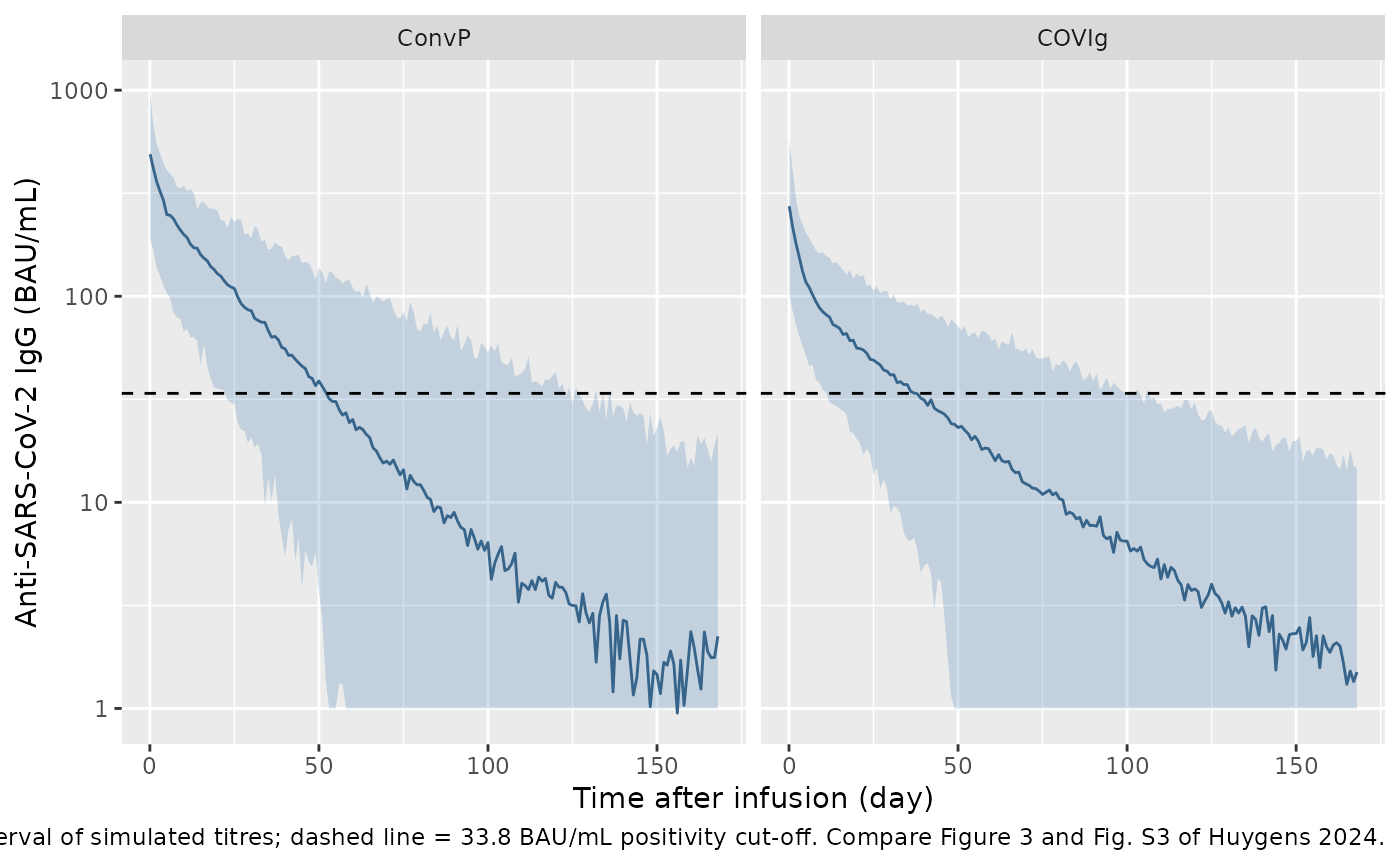
Titre-time profiles (Figure 3 and supplement Figs. S2-S3)
# Simulated 2.5th, 50th and 97.5th percentiles of the observed-scale titre
# (`sim`, including residual error) by product. Compare with the paper's
# Figure 3 pcVPC and the product-stratified supplement Figure S3 (log scale).
sim |>
  filter(time > 0) |>
  group_by(product, day) |>
  summarise(
    lo = quantile(sim, 0.025),
    med = median(sim),
    hi = quantile(sim, 0.975),
    .groups = "drop"
  ) |>
  ggplot(aes(day, med)) +
  geom_ribbon(aes(ymin = pmax(lo, 1), ymax = hi), alpha = 0.25, fill = "steelblue") +
  geom_line(colour = "steelblue4") +
  geom_hline(yintercept = 33.8, linetype = "dashed") +
  facet_wrap(~product) +
  scale_y_log10() +
  labs(
    x = "Time after infusion (day)",
    y = "Anti-SARS-CoV-2 IgG (BAU/mL)",
    caption = "Median and 95% interval of simulated titres; dashed line = 33.8 BAU/mL positivity cut-off. Compare Figure 3 and Fig. S3 of Huygens 2024."
  )
Peak titre and time to seronegativity (Table 3)
Table 3 reports, per arm, the median peak titre measured 1 hour after the infusion and the median time until the titre fell below 33.8 BAU/mL. The published times sit on the sampling schedule (41 days is about week 6, 56 days week 8, 84 days week 12), so the simulated time to seronegativity is the first protocol visit (1, 2, 4, 6, 8, 12, 18 or 24 weeks) at which the individual prediction is below the cut-off. The continuous crossing time comes 10-30 days earlier.
published_t3 <- tribble(
  ~arm, ~peak_pub, ~seroneg_pub,
  "P2", 675, 116,
  "P3", 409, 71,
  "P4", 511, 84,
  "C3", 170, 41,
  "C4", 369, 56
)

peak <- sim |>
  filter(time == inf_h + 1) |>
  group_by(arm) |>
  summarise(peak_sim = median(Cc), .groups = "drop")

seroneg <- sim |>
  filter(time %in% protocol_h, time > 48, Cc < 33.8) |>
  group_by(arm, id) |>
  summarise(t_neg = min(day), .groups = "drop") |>
  group_by(arm) |>
  summarise(seroneg_sim = median(t_neg), .groups = "drop")

t3 <- published_t3 |>
  left_join(peak, by = "arm") |>
  left_join(seroneg, by = "arm") |>
  mutate(
    peak_pct = 100 * (peak_sim / peak_pub - 1),
    seroneg_pct = 100 * (seroneg_sim / seroneg_pub - 1)
  )

t3 |>
  rename(
    "Arm" = arm,
    "Peak, published (BAU/mL)" = peak_pub,
    "Peak, simulated (BAU/mL)" = peak_sim,
    "Peak difference (%)" = peak_pct,
    "Seronegative, published (day)" = seroneg_pub,
    "Seronegative, simulated (day)" = seroneg_sim,
    "Seronegative difference (%)" = seroneg_pct
  ) |>
knitr::kable(digits = 0, caption = "Simulated vs. published median peak titre and time to seronegativity (Huygens 2024 Table 3).")| Arm | Peak, published (BAU/mL) | Seronegative, published (day) | Peak, simulated (BAU/mL) | Seronegative, simulated (day) | Peak difference (%) | Seronegative difference (%) |
|---|---|---|---|---|---|---|
| P2 | 675 | 116 | 579 | 56 | -14 | -52 |
| P3 | 409 | 71 | 245 | 42 | -40 | -41 |
| P4 | 511 | 84 | 544 | 70 | 6 | -17 |
| C3 | 170 | 41 | 175 | 35 | 3 | -15 |
| C4 | 369 | 56 | 330 | 56 | -11 | 0 |
# The two large COVIg arms (n = 11 and 19) carry the structural check on the
# peak: a mis-transcribed V1 or dose would move these medians by tens of
# percent. The ConvP arms hold three to six patients each and are not gated.
# Time to seronegativity is not gated: it is quantised to the visit schedule,
# so an arm median can jump by two weeks between virtual cohorts.
big <- t3 |> filter(arm %in% c("C3", "C4"))
stopifnot(all(abs(big$peak_pct) < 25))
The peak titres of the COVIg arms match within about 10%, and the COVIg times to seronegativity fall on or next to the published visit. The three- to six-patient ConvP arms are less well reproduced: P3’s published peak is higher than the model’s prediction for a unit at the median product titre, and all three ConvP arms stay seropositive longer than simulated. The ConvP units were single donations with widely varying titres (1100-5420 BAU/mL in supplement S4), and the patients’ own unit titres are not reported, so the simulation can only use the median. Assigning the V2 factor to ConvP instead (reading B) lengthens the simulated ConvP times towards the published ones but shortens C4, the largest arm, from 56 to 42 days; Table 3 alone therefore does not decide between the readings, and Figure 4 does.
PKNCA validation (supplement S7)
Supplement S7 gives the terminal half-life and AUC per product. The
simulated titres are sampled on the protocol schedule, values below the
33.8 BAU/mL cut-off are set to zero so that auclast stops
at the last positive sample as in the trial, and time is converted to
days to match the reported units.
sim_nca <- sim |>
  filter(!is.na(Cc), time %in% c(0, protocol_h)) |>
  mutate(Cc = ifelse(time > 0 & Cc < 33.8, 0, Cc)) |>
  select(id, day, Cc, product)

dose_df <- events |>
  filter(evid == 1) |>
  mutate(day = time / 24) |>
  select(id, day, amt, product)

conc_obj <- PKNCA::PKNCAconc(sim_nca, Cc ~ day | product + id)
dose_obj <- PKNCA::PKNCAdose(dose_df, amt ~ day | product + id)
intervals <- data.frame(
  start = 0,
  end = Inf,
  cmax = TRUE,
  auclast = TRUE,
  half.life = TRUE
)
nca_res <- PKNCA::pk.nca(PKNCA::PKNCAdata(conc_obj, dose_obj, intervals = intervals))
#> Warning: Too few points for half-life calculation (min.hl.points=3 with only 2
#> points)

published_s7 <- tribble(
  ~product, ~auclast, ~half.life,
  "ConvP", 6579, 18.6,
  "COVIg", 3458, 20.3
)

cmp <- nlmixr2lib::ncaComparisonTable(
  simulated = nca_res,
  reference = published_s7,
  by = "product",
  units = c(auclast = "BAU day/mL", half.life = "day"),
  tolerance_pct = 20
)
knitr::kable(
  cmp,
  caption = "Simulated vs. published median AUC and terminal half-life (Huygens 2024 supplement S7). * differs from reference by >20%."
)| NCA parameter | product | Reference | Simulated | % diff |
|---|---|---|---|---|
| AUClast (BAU day/mL) | ConvP | 6580 | 6530 | -0.7% |
| AUClast (BAU day/mL) | COVIg | 3460 | 2620 | -24.1%* |
| t½ (day) | ConvP | 18.6 | 16.4 | -12.0% |
| t½ (day) | COVIg | 20.3 | 19.6 | -3.7% |
The ConvP AUC and both half-lives agree with supplement S7. The simulated COVIg AUC is about a quarter below the published median. Supplement S7 does not describe how its AUC was computed (observed titres to the last positive sample, or individual model predictions), and the simulated value moves with that choice; with the same CL for both products and matching COVIg peaks, the gap is more likely a difference in method than in the model. Most of the AUC difference between the products reflects the larger doses of the ConvP arms (up to 1.9 million BAU for 600 mL, against 0.6-1.2 million BAU for COVIg), not a clearance difference: CL has no product effect in the final model.
Probability of target attainment (Figure 4)
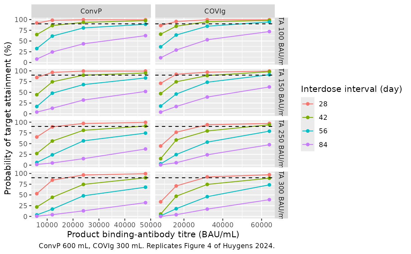
Figure 4 simulates repeated dosing of 600 mL ConvP or 300 mL COVIg at four interdose intervals and a range of product titres, and plots the fraction of patients reaching each target titre. The paper does not state the exact attainment criterion; here a patient attains the target when the steady-state trough (just before the sixth dose) is at or above it. Covariates were drawn from the study cohort in the paper; here the lean body weights of the virtual cohort above are reused.
Because the model is linear in dose, each product and interval is solved once for a product titre of 1 BAU/mL and the troughs are scaled by each titre.
pta_subjects <- subjects |>
  slice_sample(n = 200) |>
  mutate(id = row_number()) |>
  select(id, LBM)

pta_grid <- tidyr::expand_grid(
  product = c("ConvP", "COVIg"),
  tau_day = c(28, 42, 56, 84)
)

solve_trough <- function(product, tau_day) {
  vol <- if (product == "ConvP") 600 else 300
  tau <- tau_day * 24
  ev <- bind_rows(
    pta_subjects |>
      mutate(time = 0, amt = vol, rate = vol / inf_h, ii = tau, addl = 5L, evid = 1L),
    pta_subjects |>
      mutate(time = 5 * tau - 0.01, amt = 0, rate = 0, ii = 0, addl = 0L, evid = 0L)
  ) |>
    mutate(
      cmt = "central",
      FORM_SARSCOV2IGG_HYPERIMMUNE = as.integer(product == "COVIg")
    ) |>
    arrange(id, time)
  s <- rxode2::rxSolve(mod, events = ev) |> as.data.frame()
  tibble(product = product, tau_day = tau_day, trough_per_titre = s$Cc)
}
troughs <- bind_rows(Map(solve_trough, pta_grid$product, pta_grid$tau_day))

# Titres on the Figure 4 x-axis, and the 300 BAU/mL panel digitised by the
# maintainers from the published figure (percent of patients).
fig4_300 <- tribble(
  ~product, ~titre, ~tau_day, ~pta_pub,
  "ConvP", 6000, 28, 53, "ConvP", 12000, 28, 84, "ConvP", 24000, 28, 96, "ConvP", 48000, 28, 99,
  "ConvP", 6000, 42, 17, "ConvP", 12000, 42, 49, "ConvP", 24000, 42, 78, "ConvP", 48000, 42, 92,
  "ConvP", 6000, 56, 5, "ConvP", 12000, 56, 22, "ConvP", 24000, 56, 50, "ConvP", 48000, 56, 75,
  "ConvP", 6000, 84, 1, "ConvP", 12000, 84, 3, "ConvP", 24000, 84, 14, "ConvP", 48000, 84, 34,
  "COVIg", 8000, 28, 36, "COVIg", 16000, 28, 77, "COVIg", 32000, 28, 94, "COVIg", 64000, 28, 99,
  "COVIg", 8000, 42, 10, "COVIg", 16000, 42, 41, "COVIg", 32000, 42, 76, "COVIg", 64000, 42, 93,
  "COVIg", 8000, 56, 3, "COVIg", 16000, 56, 17, "COVIg", 32000, 56, 49, "COVIg", 64000, 56, 78,
  "COVIg", 8000, 84, 1, "COVIg", 16000, 84, 3, "COVIg", 32000, 84, 16, "COVIg", 64000, 84, 39
)

pta <- tidyr::expand_grid(
  target = c(100, 150, 250, 300),
  distinct(fig4_300, product, titre)
) |>
  left_join(troughs, by = "product", relationship = "many-to-many") |>
  group_by(target, product, titre, tau_day) |>
  summarise(pta = 100 * mean(trough_per_titre * titre >= target), .groups = "drop")

ggplot(pta, aes(titre, pta, colour = factor(tau_day))) +
  geom_line() +
  geom_point() +
  geom_hline(yintercept = 90, linetype = "dashed") +
  facet_grid(paste("PTA", target, "BAU/mL") ~ product, scales = "free_x") +
  labs(
    x = "Product binding-antibody titre (BAU/mL)",
    y = "Probability of target attainment (%)",
    colour = "Interdose interval (day)",
    caption = "ConvP 600 mL, COVIg 300 mL. Replicates Figure 4 of Huygens 2024."
  )
pta_cmp <- fig4_300 |>
  left_join(filter(pta, target == 300), by = c("product", "titre", "tau_day")) |>
  mutate(diff = pta - pta_pub)

pta_cmp |>
  select(product, tau_day, titre, pta_pub, pta, diff) |>
  rename(
    "Product" = product,
    "Interval (day)" = tau_day,
    "Titre (BAU/mL)" = titre,
    "PTA, Figure 4 (%)" = pta_pub,
    "PTA, simulated (%)" = pta,
    "Difference (points)" = diff
  ) |>
knitr::kable(digits = 0, caption = "300 BAU/mL target: simulated vs. digitised Figure 4.")| Product | Interval (day) | Titre (BAU/mL) | PTA, Figure 4 (%) | PTA, simulated (%) | Difference (points) |
|---|---|---|---|---|---|
| ConvP | 28 | 6000 | 53 | 53 | 0 |
| ConvP | 28 | 12000 | 84 | 84 | 0 |
| ConvP | 28 | 24000 | 96 | 96 | 0 |
| ConvP | 28 | 48000 | 99 | 100 | 0 |
| ConvP | 42 | 6000 | 17 | 22 | 5 |
| ConvP | 42 | 12000 | 49 | 44 | -4 |
| ConvP | 42 | 24000 | 78 | 74 | -4 |
| ConvP | 42 | 48000 | 92 | 90 | -2 |
| ConvP | 56 | 6000 | 5 | 4 | -1 |
| ConvP | 56 | 12000 | 22 | 17 | -5 |
| ConvP | 56 | 24000 | 50 | 48 | -2 |
| ConvP | 56 | 48000 | 75 | 68 | -7 |
| ConvP | 84 | 6000 | 1 | 0 | 0 |
| ConvP | 84 | 12000 | 3 | 4 | 1 |
| ConvP | 84 | 24000 | 14 | 13 | -1 |
| ConvP | 84 | 48000 | 34 | 32 | -2 |
| COVIg | 28 | 8000 | 36 | 34 | -2 |
| COVIg | 28 | 16000 | 77 | 71 | -6 |
| COVIg | 28 | 32000 | 94 | 92 | -2 |
| COVIg | 28 | 64000 | 99 | 97 | -2 |
| COVIg | 42 | 8000 | 10 | 6 | -4 |
| COVIg | 42 | 16000 | 41 | 47 | 6 |
| COVIg | 42 | 32000 | 76 | 74 | -2 |
| COVIg | 42 | 64000 | 93 | 89 | -4 |
| COVIg | 56 | 8000 | 3 | 2 | -2 |
| COVIg | 56 | 16000 | 17 | 18 | 1 |
| COVIg | 56 | 32000 | 49 | 46 | -3 |
| COVIg | 56 | 64000 | 78 | 74 | -4 |
| COVIg | 84 | 8000 | 1 | 0 | -1 |
| COVIg | 84 | 16000 | 3 | 4 | 1 |
| COVIg | 84 | 32000 | 16 | 17 | 1 |
| COVIg | 84 | 64000 | 39 | 39 | 0 |
# Robust envelope over the 32 points. This model gives a median absolute
# difference of about 2 points and a 90th percentile of about 5. Under the
# opposite reading of the V2 covariate (factor on ConvP) they are about 7 and
# 18 points, with single points off by up to 21, so the gate discriminates
# between the readings while leaving room for Monte Carlo noise (about 3.5
# points at 50% attainment with 200 subjects).
stopifnot(
  median(abs(pta_cmp$diff)) < 4.5,
  quantile(abs(pta_cmp$diff), 0.9) < 10
)
The text’s key conclusions are reproduced: 600 mL ConvP every 8 weeks does not reach 90% attainment of 300 BAU/mL at any titre shown, while monthly dosing reaches it from roughly 12,000-24,000 BAU/mL. Per BAU infused, COVIg attains the targets slightly more often than ConvP (compare COVIg 16,000 BAU/mL x 300 mL with ConvP 6,000-12,000 BAU/mL x 600 mL), which follows from its larger V2 and longer terminal phase.
Assumptions and deviations
- V2 covariate direction. The printed equation (factor 1.99 on V2 for COVIg) is used rather than the prose (factor on ConvP); the base-model V2, the supplement S7 half-lives and Figure 4 all support the equation. See the section above.
- Lean body weight formula. The paper uses lean body weight with a 70 kg reference but does not name the formula or report the cohort distribution. The virtual cohort uses the James formula. The base-model V1 (3340 mL) equals the final-model V1 at a lean body weight of about 55 kg, consistent with this cohort.
- IIV scale. Table 2 reports IIV as %CV; variances were computed as log(CV^2 + 1).
- Residual error. The mixed error model is encoded as additive (3.75 BAU/mL) plus proportional (9.68%) standard deviations.
- Dose. Each arm’s dose is the median CLIA titre of its product (3230, 3070 and 3985 BAU/mL) times the infused volume. Individual ConvP units varied widely, which the median cannot capture.
- Infusion duration. Not reported; a 1-hour infusion is assumed. Over a multi-week profile the choice is immaterial.
- Figure 4 criterion. Target attainment is taken as the steady-state trough (before the sixth dose) at or above the target, without residual error; the paper does not specify the criterion.
- Body size by arm. Per-arm sex fraction and median weight and height come from supplement S6; the spread (lognormal weight SD 0.18, height SD 7 cm) is assumed.
- No erratum or correction notice for this article was found as of 2026-10-29.