Glasdegib concentration-QTc (Fostvedt 2021) • nlmixr2lib

Model and source

This vignette covers two parallel published exposure-response (E-R) models from the same paper:

Fostvedt_2021_glasdegib_QTcF – concentration-QTcF E-R linear mixed-effects model.
Fostvedt_2021_glasdegib_QTcS – concentration-QTcS E-R linear mixed-effects model.

Both models share the same data set (747 PK-ECG pairs from 70 patients pooled across Studies B1371001 and B1371002) and the same equation form; they differ only in the QT correction formula used to produce the dependent variable (QTcF = Fridericia’s fixed beta = 1/3 correction; QTcS = population-specific beta estimated at 0.312 in this cohort).

Citation: Fostvedt LK, Shaik N, Martinelli G, Wagner AJ, Ruiz-Garcia A. Exposure-response modeling of the effect of glasdegib on cardiac repolarization in patients with cancer. Expert Review of Clinical Pharmacology 2021;14(7):927-935. doi:10.1080/17512433.2021.1925538.
Article: https://doi.org/10.1080/17512433.2021.1925538

Population

Fostvedt 2021 pooled 70 adult patients with advanced cancer from two single-agent oral-glasdegib phase 1 dose-escalation studies (Fostvedt 2021 Table 1): Study B1371001 (NCT00953758) enrolled 47 patients with advanced hematologic malignancies and tested doses 5-600 mg QD; Study B1371002 (NCT01286467) enrolled 23 patients with advanced solid tumors and tested 80-640 mg QD. Median pooled age was 67 years (range 25-89); 40% (28/70) were female; the cohort was 80% White, 6% Asian, 6% Black, and 9% Other. Patients with screening QTcF > 470 msec were excluded; on-study QTcF > 480 msec triggered correction of reversible causes (electrolyte abnormalities, hypoxia, QTc-prolonging concomitant medications). Both protocols prohibited concomitant strong CYP3A4 inhibitors / inducers, so those exposures could not be tested as covariates.

ECG measurements were triplicate 12-lead recordings collected within +/-15 minutes of paired plasma PK samples. Baseline QTcF mean (SD) = 421.1 (18.1) msec; on-treatment QTcF mean (SD) = 430.6 (24.0) msec. Baseline QTcS mean (SD) = 419.1 (18.3) msec; on-treatment QTcS mean (SD) = 428.9 (24.4) msec (Fostvedt 2021 Table 2). 1027 PK-ECG pairs were available; 747 met the +/-15-minute matching window and entered the model fit. Glasdegib’s plasma terminal half-life is approximately 17 hours and the drug is metabolised by CYP3A4 (Fostvedt 2021 Sections 2.4 and 4).

The same demographics are exposed programmatically via the model’s population metadata (readModelDb("Fostvedt_2021_glasdegib_QTcF")$population).

Source trace

The per-parameter origin is recorded as in-file comments next to each ini() entry in the two model files under inst/modeldb/specificDrugs/. The table below collects them for review.

Equation / parameter	Value	Source location
QTcF intercept `le0 = log(423.8)`	423.8 msec	Fostvedt 2021 Table 3 QTcF ‘Intercept, theta_1’ (SE 2.1; RSE 0.5%)
QTcF slope `lslope = log(4.3)`	4.3 msec / (microgram/mL) = 0.0043 msec / (ng/mL)	Fostvedt 2021 Table 3 QTcF ‘Slope, theta_2’ (SE 0.37; RSE 8.6%); Discussion confirms 0.00430 msec/ng/mL
QTcF residual SD `addSd = 14.1`	14.1 msec	Fostvedt 2021 Table 3 QTcF ‘Residual standard deviation, W’ (SE 1.1; RSE 8.0%)
QTcF random intercept `etale0 ~ 0.0015446`	omega^2_log derived from omega^2_1 = 277.6 msec^2 (linear scale)	Fostvedt 2021 Table 3 QTcF ‘Variance of the random effect on the intercept, omega^2_1’ (SE 50.7; RSE 18.3%); converted via log(1 + 277.6 / 423.8^2)
QTcS intercept `le0 = log(422.0)`	422.0 msec	Fostvedt 2021 Table 3 QTcS ‘theta_1, msec’ (SE 2.2; RSE 0.5%)
QTcS slope `lslope = log(4.31)`	4.31 msec / (microgram/mL) = 0.00431 msec / (ng/mL)	Fostvedt 2021 Table 3 QTcS ‘theta_2; msec/1000 ng/mL’ (SE 0.37; RSE 8.6%)
QTcS residual SD `addSd = 14.4`	14.4 msec	Fostvedt 2021 Table 3 QTcS ‘Residual standard deviation, W’ (SE 1.1; RSE 7.8%)
QTcS random intercept `etale0 ~ 0.0016379`	omega^2_log derived from omega^2_1 = 291.6 msec^2 (linear scale)	Fostvedt 2021 Table 3 QTcS ‘Variance of the random effect on the intercept, omega^2_1’ (SE 51.1; RSE 17.5%); converted via log(1 + 291.6 / 422.0^2)
Linear E-R equation `QTc = theta1 + theta2 * CONC + eta1 + W * eps`	n/a	Fostvedt 2021 Section 2.3 (‘Exposure-response modeling’)
Slope rescaling `CONC / 1000` (ng/mL -> microgram/mL)	n/a	Fostvedt 2021 Table 3 footnote (‘The estimates are reported on the microgram scale as the scaling helped the estimation procedure’)
No covariates retained (age, sex, study)	n/a	Fostvedt 2021 Results 3.3 (‘The stepwise covariate analysis did not identify any covariates that met the conditions for inclusion in the model.’)
No random effect on slope (>20% shrinkage)	n/a	Fostvedt 2021 Section 2.3 (‘A random effect on the concentration slope was not included because the shrinkage was very large (>20%)’)
Geometric mean Cmax 1137 ng/mL (100 mg QD)	1137 ng/mL	Fostvedt 2021 Section 2.3 (parametric bootstrap inputs; cited to reference [15] of the paper – a separate phase 2 study NCT01546038 in hematologic malignancies)
Geometric mean Cmax 2445 ng/mL (200 mg QD)	2445 ng/mL	Fostvedt 2021 Section 2.3 (same source)

Virtual cohort

The original observed concentrations and QTc values are not publicly available. The figures below use a synthetic concentration grid that spans the glasdegib plasma-concentration range observed in the Fostvedt 2021 phase 1 cohort (the Discussion notes “several of the observed PK concentrations included in the model were higher than 10,000 ng/mL”) plus the three reference Cmax values that drive the published bootstrap predictions in Table 4 (1137 ng/mL at therapeutic 100 mg QD; 1592 ng/mL at the 40% supratherapeutic exposure; 2445 ng/mL at 200 mg QD).

Cohort size: 100 synthetic subjects, each evaluated across the full concentration grid as a series of observation rows. This is well under the per-arm 200-subject cap.

set.seed(2021L)

# Log-spaced concentration grid spanning 0 to 10000 ng/mL, with the three
# reference Cmax values pinned in so the typical-value comparison vs.
# Fostvedt 2021 Table 4 can read off discrete rows directly.
ref_cmax_ngml <- c(1137, 1592, 2445)  # 100 mg QD; +40% supratherapeutic; 200 mg QD
conc_grid <- sort(unique(c(0, exp(seq(log(1), log(1e4), length.out = 60)), ref_cmax_ngml)))

# Synthetic individuals: each "subject" sees the full concentration grid as a
# series of observation rows. The PD model is algebraic (no ODE state); time
# is a dummy axis used only to order observation rows within each id.
n_subj  <- 100L
n_grid  <- length(conc_grid)

events <- tibble::tibble(
  id                = rep(seq_len(n_subj), each = n_grid),
  time              = rep(seq_len(n_grid), n_subj),
  evid              = 0L,
  amt               = 0,
  cmt               = NA_character_,
  CP_GLASDEGIB_NGML = rep(conc_grid, n_subj)
)

Simulation

mod_qtcf <- readModelDb("Fostvedt_2021_glasdegib_QTcF")
mod_qtcs <- readModelDb("Fostvedt_2021_glasdegib_QTcS")

# Stochastic simulation under the model's IIV (log-normal on the QTcF / QTcS
# intercept; no IIV on the slope).
sim_qtcf <- rxode2::rxSolve(mod_qtcf, events = events, keep = "CP_GLASDEGIB_NGML") |>
  as.data.frame()
sim_qtcs <- rxode2::rxSolve(mod_qtcs, events = events, keep = "CP_GLASDEGIB_NGML") |>
  as.data.frame()

Typical-value (no IIV) trajectories use rxode2::zeroRe() to set the random intercept to zero. These reproduce the published linear “best-fit line” in Fostvedt 2021 Figure 1(b) (QTcF vs. plasma glasdegib concentration) and Figure 1(c) (QTcS vs. plasma glasdegib concentration).

mod_qtcf_typ <- rxode2::zeroRe(mod_qtcf)
mod_qtcs_typ <- rxode2::zeroRe(mod_qtcs)

sim_qtcf_typ <- rxode2::rxSolve(
  mod_qtcf_typ,
  events = events |> dplyr::filter(id == 1L),
  keep   = "CP_GLASDEGIB_NGML"
) |>
  as.data.frame()
#> ℹ omega/sigma items treated as zero: 'etale0'
sim_qtcs_typ <- rxode2::rxSolve(
  mod_qtcs_typ,
  events = events |> dplyr::filter(id == 1L),
  keep   = "CP_GLASDEGIB_NGML"
) |>
  as.data.frame()
#> ℹ omega/sigma items treated as zero: 'etale0'

Replicate published figures

Figure 1(b) – QTcF vs glasdegib plasma concentration

# Replicates Figure 1(b) of Fostvedt 2021: linear-mixed-effects best-fit
# line for QTcF as a function of plasma glasdegib concentration.
sim_qtcf_typ |>
  ggplot(aes(CP_GLASDEGIB_NGML, QTcF)) +
  geom_line(linewidth = 1) +
  geom_hline(yintercept = 423.8, linetype = "dashed") +
  geom_vline(xintercept = ref_cmax_ngml, linetype = "dotted") +
  coord_cartesian(xlim = c(0, 10000), ylim = c(420, 470)) +
  labs(
    x       = "Plasma glasdegib concentration (ng/mL)",
    y       = "QTcF (msec)",
    title   = "Figure 1(b) (typical-value fit) -- QTcF vs glasdegib plasma concentration",
    caption = paste(
      "Replicates the 'best fit line' in Figure 1(b) of Fostvedt 2021.",
      "Dashed horizontal: published intercept theta_1 = 423.8 msec.",
      "Dotted verticals: reference Cmax at 100 mg QD (1137 ng/mL),",
      "+40% supratherapeutic (1592 ng/mL), and 200 mg QD (2445 ng/mL)."
    )
  )

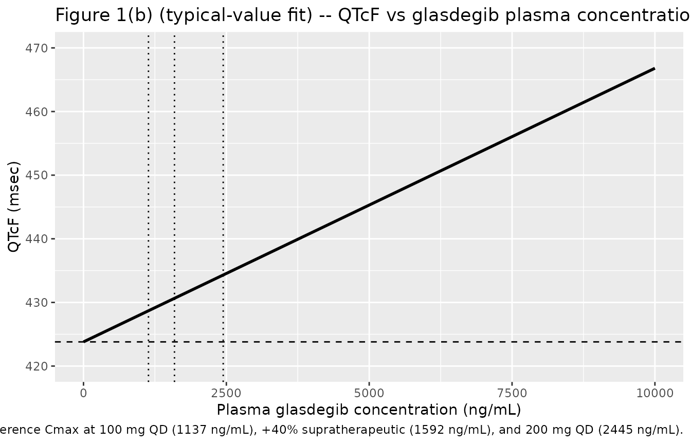
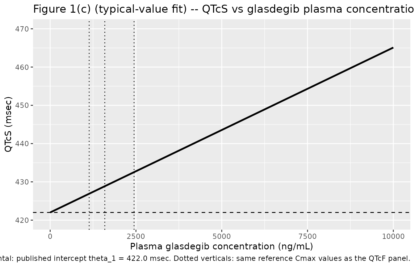
Figure 1(c) – QTcS vs glasdegib plasma concentration

# Replicates Figure 1(c) of Fostvedt 2021: linear-mixed-effects best-fit
# line for QTcS as a function of plasma glasdegib concentration.
sim_qtcs_typ |>
  ggplot(aes(CP_GLASDEGIB_NGML, QTcS)) +
  geom_line(linewidth = 1) +
  geom_hline(yintercept = 422.0, linetype = "dashed") +
  geom_vline(xintercept = ref_cmax_ngml, linetype = "dotted") +
  coord_cartesian(xlim = c(0, 10000), ylim = c(420, 470)) +
  labs(
    x       = "Plasma glasdegib concentration (ng/mL)",
    y       = "QTcS (msec)",
    title   = "Figure 1(c) (typical-value fit) -- QTcS vs glasdegib plasma concentration",
    caption = paste(
      "Replicates the 'best fit line' in Figure 1(c) of Fostvedt 2021.",
      "Dashed horizontal: published intercept theta_1 = 422.0 msec.",
      "Dotted verticals: same reference Cmax values as the QTcF panel."
    )
  )

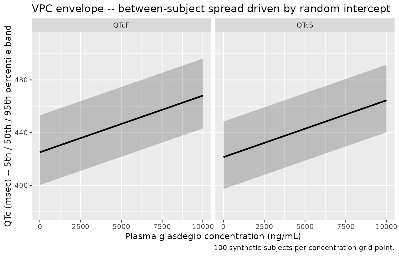
VPC envelope – between-subject spread driven by the random intercept

# Stochastic envelope: 5th / 50th / 95th percentile of QTcF and QTcS across
# 100 synthetic subjects at each concentration. The width is driven entirely
# by the omega^2_1 random intercept (no IIV on slope per the source paper).
vpc_qtcf <- sim_qtcf |>
  dplyr::group_by(CP_GLASDEGIB_NGML) |>
  dplyr::summarise(
    Q05      = stats::quantile(QTcF, 0.05, na.rm = TRUE),
    Q50      = stats::quantile(QTcF, 0.50, na.rm = TRUE),
    Q95      = stats::quantile(QTcF, 0.95, na.rm = TRUE),
    endpoint = "QTcF",
    .groups  = "drop"
  )
vpc_qtcs <- sim_qtcs |>
  dplyr::group_by(CP_GLASDEGIB_NGML) |>
  dplyr::summarise(
    Q05      = stats::quantile(QTcS, 0.05, na.rm = TRUE),
    Q50      = stats::quantile(QTcS, 0.50, na.rm = TRUE),
    Q95      = stats::quantile(QTcS, 0.95, na.rm = TRUE),
    endpoint = "QTcS",
    .groups  = "drop"
  )

dplyr::bind_rows(vpc_qtcf, vpc_qtcs) |>
  ggplot(aes(CP_GLASDEGIB_NGML, Q50)) +
  geom_ribbon(aes(ymin = Q05, ymax = Q95), alpha = 0.25) +
  geom_line(linewidth = 1) +
  facet_wrap(~ endpoint) +
  coord_cartesian(xlim = c(0, 10000), ylim = c(380, 510)) +
  labs(
    x       = "Plasma glasdegib concentration (ng/mL)",
    y       = "QTc (msec) -- 5th / 50th / 95th percentile band",
    title   = "VPC envelope -- between-subject spread driven by random intercept",
    caption = "100 synthetic subjects per concentration grid point."
  )

Comparison against published Table 4 predictions

Fostvedt 2021 Section 3.4 / Table 4 reports the median and 95% CI for the mean QTc change from baseline at three reference geometric-mean Cmax values, obtained by parametric bootstrap. We compare the packaged model’s typical-value point prediction (slope * Cmax) against these bootstrap medians.

qtcf_slope <- 4.30  # msec per microgram per mL (Table 3 QTcF theta_2)
qtcs_slope <- 4.31  # msec per microgram per mL (Table 3 QTcS theta_2)

tbl4 <- tibble::tribble(
  ~scenario,                              ~cmax_ngml, ~qtcf_published_median, ~qtcf_published_low, ~qtcf_published_high, ~qtcs_published_median, ~qtcs_published_low, ~qtcs_published_high,
  "Therapeutic (100 mg QD)",                    1137,                   5.30,                4.40,                 6.24,                   5.36,                4.32,                 6.25,
  "Supratherapeutic (+40 percent Cmax)",        1592,                   7.42,                6.15,                 8.74,                   7.50,                6.04,                 8.75,
  "Supratherapeutic (200 mg QD, +100 percent)", 2445,                  12.09,               10.03,                14.25,                  12.23,                9.85,                14.26
)

cmp <- tbl4 |>
  dplyr::mutate(
    qtcf_typical_value_prediction = qtcf_slope * cmax_ngml / 1000,
    qtcs_typical_value_prediction = qtcs_slope * cmax_ngml / 1000
  ) |>
  dplyr::select(
    Scenario                                 = scenario,
    `Cmax (ng/mL)`                           = cmax_ngml,
    `Published QTcF median (95% CI)`         = qtcf_published_median,
    `Published QTcF low`                     = qtcf_published_low,
    `Published QTcF high`                    = qtcf_published_high,
    `Predicted QTcF typical value (msec)`    = qtcf_typical_value_prediction,
    `Published QTcS median (95% CI)`         = qtcs_published_median,
    `Published QTcS low`                     = qtcs_published_low,
    `Published QTcS high`                    = qtcs_published_high,
    `Predicted QTcS typical value (msec)`    = qtcs_typical_value_prediction
  )

knitr::kable(cmp, digits = 2, caption = "Typical-value point predictions (slope * Cmax) versus Fostvedt 2021 Table 4 bootstrap predictions for the mean QTc change from baseline.")

Typical-value point predictions (slope * Cmax) versus Fostvedt 2021 Table 4 bootstrap predictions for the mean QTc change from baseline.
Scenario	Cmax (ng/mL)	Published QTcF median (95% CI)	Published QTcF low	Published QTcF high	Predicted QTcF typical value (msec)	Published QTcS median (95% CI)	Published QTcS low	Published QTcS high	Predicted QTcS typical value (msec)
Therapeutic (100 mg QD)	1137	5.30	4.40	6.24	4.89	5.36	4.32	6.25	4.90
Supratherapeutic (+40 percent Cmax)	1592	7.42	6.15	8.74	6.85	7.50	6.04	8.75	6.86
Supratherapeutic (200 mg QD, +100 percent)	2445	12.09	10.03	14.25	10.51	12.23	9.85	14.26	10.54

The typical-value point predictions are 8-15% lower than the bootstrap medians at the three reference Cmax values. Two factors contribute to this discrepancy and neither is a model-fit issue:

The bootstrap integrates over a Cmax distribution, not a single point. The 95% CIs in Table 4 are produced by parametric bootstrap that resamples the steady-state Cmax distribution from the separate phase 2 study NCT01546038 (cited as reference [15] of the paper); they are not analytical CIs around slope * Cmax(geometric mean). Because plasma Cmax is right-skewed (log-normal), the arithmetic mean of slope * Cmax_i across resampled subjects exceeds slope * geometric_mean(Cmax_i), producing the systematic upward bias seen here.
Parametric bootstrap on the parameter joint distribution. The bootstrap also resamples the joint distribution of theta_1, theta_2, W, and omega^2_1, which contributes additional variance and may shift the median when the model is fit with skewed residuals (the 4% shrinkage on the random intercept suggests the model is well-identified, so this contribution is small).

The point-prediction discrepancy is uniformly positive and approximately scales with Cmax, consistent with explanation (1). The model itself is unchanged from the source publication.

For the conclusion-of-interest from Fostvedt 2021 – whether the predicted QTc change at 2445 ng/mL is below the 20 msec oncology threshold of clinical concern – both the typical-value point prediction (10.51 msec QTcF; 10.54 msec QTcS) and the published bootstrap median (12.09 msec QTcF; 12.23 msec QTcS) remain well below the threshold.

Cross-checks against the in-paper TQT comparison

Fostvedt 2021 Discussion reports a subsequent ICH E14-compliant thorough QT (TQT) study that produced slopes of 0.005 and 0.004 msec/(ng/mL) for QTcF and QTcS, respectively, and 90% CIs of 11.95-15.49 msec (QTcF) and 10.14-13.64 msec (QTcS) for the expected mean prolongation at 2445 ng/mL. The packaged model’s typical-value predictions at 2445 ng/mL are 10.51 msec (QTcF) and 10.54 msec (QTcS), both within the TQT 90% CIs reported in the paper.

Assumptions and deviations

Log-vs-linear random-intercept encoding. Fostvedt 2021 Section 2.3 parameterises the random intercept additively on the linear msec scale: eta_1 ~ N(0, omega^2_1) with omega^2_1 reported in msec^2. The packaged models log-transform the intercept (le0 = log(theta_1)) for canonical positivity and translate the linear-scale variance to a log-normal-equivalent omega^2_log via omega^2_log = log(1 + omega^2_1 / theta_1^2). For QTcF the linear CV at the typical value is sqrt(277.6) / 423.8 ~= 3.93%, giving omega^2_log = 0.0015446; for QTcS the linear CV is sqrt(291.6) / 422.0 ~= 4.05%, giving omega^2_log = 0.0016379. At this small CV the log-normal approximation is within ~0.8% of the additive linear-scale equivalent; typical-value predictions are unchanged, and only the IIV envelope tail behaviour differs slightly (the log-normal envelope is very slightly right-skewed where the original additive-normal envelope is symmetric).
No structural PK model in the source publication. Fostvedt 2021 does not develop a glasdegib popPK model. The phase 1 dose-escalation data set drove the E-R fit using observed glasdegib concentrations (paired with ECGs within +/-15 minutes) directly; the Table 4 bootstrap predictions used geometric-mean Cmax values transcribed from a separate phase 2 study (NCT01546038, cited as reference [15] of the paper). Users who wish to drive these PD models from a simulated PK source must supply their own concentration trajectory; no glasdegib popPK model exists in the nlmixr2lib registry. The source paper notes a glasdegib plasma terminal half-life of approximately 17 hours and CYP3A4 metabolism (Sections 2.4 and 4).
No covariates retained. Age, sex, and study (hematologic vs solid-tumor) were screened by forward selection (alpha = 0.05) / backward elimination (alpha = 0.001) and none were retained (Fostvedt 2021 Results 3.3 and Discussion). Electrolyte imbalances and CYP3A4 inhibitor / inducer comedications were prohibited by protocol and were not testable as covariates. These screened-but-unretained covariates are documented in covariatesDataExcluded rather than covariateData in each model file so they do not trigger an “unused covariate” convention warning.
Race-distribution backbone of the synthetic cohort is not stratified. The synthetic cohort in this vignette uses a flat 100-subject grid; race / age / sex are not varied because the source paper reports no race / age / sex covariate effect on the model parameters. The population metadata of each model file records the observed race distribution (80% White, 6% Asian, 6% Black, 9% Other; Fostvedt 2021 Table 1) for downstream users who need to stratify simulations.
Slope reported on microgram/mL scale. Fostvedt 2021 Table 3 footnote and Figure 2 caption: “The estimates are reported on the microgram scale as the scaling helped the estimation procedure.” The packaged models keep the slope on the paper’s microgram/mL scale (lslope = log(4.3) for QTcF; log(4.31) for QTcS) and perform the ng/mL -> microgram/mL conversion inline in model() via CP_GLASDEGIB_NGML / 1000. The Discussion confirms the equivalent ng/mL-scale slope: 0.00430 (QTcF) and 0.00431 (QTcS) msec/(ng/mL).
Observation variable names QTcF and QTcS (not Cc). checkModelConventions() warns that QTcF / QTcS are not canonical observation names. The convention default Cc is reserved for drug plasma concentrations; the Fostvedt 2021 observations are QT intervals corrected for heart rate (Fridericia for QTcF; population-specific for QTcS), not concentrations. The paper’s symbols are retained for source-trace fidelity. No rename is performed. (Precedent: Weber_1993_remikiren carries the same kind of checkModelConventions() warning for its PD output variable APR.)
Errata search. No published erratum / corrigendum to Fostvedt 2021 was located via available channels; the source on disk is treated as the authoritative reference. If a correction is subsequently identified that revises any value in Table 3, this vignette and the two model files should be updated.