Cyclosporine, phenobarbital and vancomycin in children: size and maturation (Back 2019)

Model and source

Back et al. (2019) fitted three independent one-compartment population PK models to three retrospective Korean paediatric therapeutic-drug-monitoring datasets, to compare an allometric size function alone with size plus a sigmoidal maturation function. Each drug is its own model file:

• Back_2019_cyclosporine: One-compartment population PK model for intravenous high-dose cyclosporine A in Korean infants and children with retinoblastoma (Back 2019), with allometric size scaling on CL (exponent 0.75) and Vd (exponent 1) referenced to 70 kg and no maturation function (not significant for this cohort).
• Back_2019_phenobarbital: One-compartment population PK model for oral and intravenous phenobarbital in Korean preterm and term neonates and infants (Back 2019), with first-order absorption, allometric size scaling on CL (exponent 0.75) and Vd (exponent 1) referenced to 70 kg, and an estimated sigmoidal postmenstrual-age maturation function on CL. The printed Vd (5.51 L at 70 kg, about 0.08 L/kg) gives an 11-h half-life in the typical neonate, which does not reproduce the flat trough profile of the paper’s own VPC (Figure 3b); the Table 3 values are encoded verbatim (see vignette Errata).
• Back_2019_vancomycin: One-compartment population PK model for intravenous vancomycin in Korean preterm neonates to infants (Back 2019), with allometric size scaling on CL (exponent 0.75) and Vd (exponent 1) referenced to 70 kg and a sigmoidal postmenstrual-age maturation function on CL with TM50 and Hill held at reference values. The printed CL (69.4 L/h) and Vd (3.23 L) at 70 kg give a 1.3-min half-life in the typical neonate and do not reproduce the paper’s own VPC (Figure 3c); the Table 3 values are encoded verbatim (see vignette Errata).
• Citation: Back HM, Lee JB, Han N, Goo S, Jung E, Kim J, Song B, An SH, Kim JT, Rhie SJ, Ree YS, Chae JW, Kim JW, Yun HY. Application of Size and Maturation Functions to Population Pharmacokinetic Modeling of Pediatric Patients. Pharmaceutics. 2019;11(6):259. doi:10.3390/pharmaceutics11060259
• Article (open access): https://doi.org/10.3390/pharmaceutics11060259

Read the Errata section before using the phenobarbital or vancomycin model. Two of the three published parameter sets do not reproduce the paper’s own visual predictive check. All three are encoded exactly as printed in Table 3.

Population

All three cohorts are single-centre Korean hospital cohorts (Back 2019 Table 1):

• Cyclosporine A (CsA): 34 infants and children (20 male, 14 female) with retinoblastoma at Yonsei University Hospital, postnatal age 26.8 +/- 17.8 (1-79) months, weight 12.9 +/- 3.8 (5-24) kg. High-dose CsA was infused over 24 h, starting 3 h before chemotherapy on days 1 and 2, as a P-glycoprotein inhibitor; samples were drawn 20 h after the start of each infusion.
• Phenobarbital (PHB): 28 preterm and term neonates and infants (11 male, 17 female) in the Kyunghee University NICU, gestational age 36.7 +/- 4.4 weeks, postnatal age 32.4 +/- 30.7 (3-150) days, post-conceptional age 41.3 +/- 3.9 (31-51.1) weeks, weight 3.3 +/- 1 (1-6.9) kg. Loading dose 15-20 mg/kg, then 3-5 mg/kg/day from 12-24 h later, oral or intravenous; troughs between 5 min and 3 h before the next dose.
• Vancomycin (VAN): 93 preterm neonates to infants (57 male, 36 female) at Chungnam National University Hospital, gestational age 31.9 +/- 4.7 weeks, postnatal age 9.3 +/- 12.4 (0.1-80.4) weeks, post-conceptional age 41.2 +/- 14.2 (25.6-110) weeks, weight 3.2 +/- 2.6 (0.4-14.9) kg. Weight-based intravenous doses every 6-24 h; samples 0.5-23.5 h after a dose.

The same information is available programmatically, e.g. readModelDb("Back_2019_vancomycin")()$population.

Source trace

The paper’s post-conceptional age (PCA) is gestational age plus postnatal age (Table 1: 36.7 weeks + 32.4 days = 41.3 weeks), i.e. the standard postmenstrual age, supplied in the canonical PAGE column in weeks.

Equation / parameter	CsA	PHB	VAN	Source location
Structure	1-cmt IV	1-cmt, first-order oral absorption + IV	1-cmt IV	Results 3.2; Figure 1
Vd = TVVd * (WT/70)^1 * exp(eta)	yes	yes	yes	Eq 4 and Eq 7; WTnormal = 70 kg (Methods 2.4)
CL = TVCL * (WT/70)^0.75 * Fmat * exp(eta)	no Fmat	yes	yes	Eq 8 (two-branch)
Fmat = PCA^Hill / (PCA^Hill + TM50^Hill)	–	yes	yes	Eq 2, Eq 5, Eq 8
lcl (CL at 70 kg, L/h)	21.3	0.569	69.4	Table 3
lvc (Vd at 70 kg, L)	218	5.51	3.23	Table 3
TM50 (weeks)	–	48.2 (ltmat50)	33.3, held constant (tmat50)	Table 3 and footnote
Hill	–	5.99 (lhill_mat)	3.68, held constant (hill_mat)	Table 3 and footnote
lka (1/h)	–	50, held constant	–	Table 3
lfdepot	–	0.724	–	Table 3
e_wt_cl, e_wt_vc	0.75, 1	0.75, 1	0.75, 1	Eq 7, Eq 8 (printed exponents)
IIV CL (CV) -> etalcl variance	16.8% -> 0.02783	40.8% -> 0.154	10.4% -> 0.01076	Table 3; log(CV^2 + 1)
IIV Vd (CV) -> etalvc variance	12.3% -> 0.01502	78.7% -> 0.482	52.8% -> 0.2459	Table 3; log(CV^2 + 1)
propSd	0.468	0.356	0.408	Table 3; Eq 6 (CCV model)

ui <- list(
  CsA = rxode2::rxode(readModelDb("Back_2019_cyclosporine")),
  PHB = rxode2::rxode(readModelDb("Back_2019_phenobarbital")),
  VAN = rxode2::rxode(readModelDb("Back_2019_vancomycin"))
)
#> ℹ parameter labels from comments will be replaced by 'label()'
#> ℹ parameter labels from comments will be replaced by 'label()'
#> ℹ parameter labels from comments will be replaced by 'label()'
th <- lapply(ui, function(u) u$theta)

# Every structural value against Back 2019 Table 3, on the scale printed there.
table3 <- tibble::tribble(
  ~drug, ~param,      ~printed, ~encoded,
  "CsA", "CL (L/h)",  21.3,     exp(th$CsA[["lcl"]]),
  "CsA", "Vd (L)",    218,      exp(th$CsA[["lvc"]]),
  "CsA", "prop err",  0.468,    th$CsA[["propSd"]],
  "PHB", "CL (L/h)",  0.569,    exp(th$PHB[["lcl"]]),
  "PHB", "Vd (L)",    5.51,     exp(th$PHB[["lvc"]]),
  "PHB", "TM50 (wk)", 48.2,     exp(th$PHB[["ltmat50"]]),
  "PHB", "Hill",      5.99,     exp(th$PHB[["lhill_mat"]]),
  "PHB", "ka (1/h)",  50,       exp(th$PHB[["lka"]]),
  "PHB", "F",         0.724,    exp(th$PHB[["lfdepot"]]),
  "PHB", "prop err",  0.356,    th$PHB[["propSd"]],
  "VAN", "CL (L/h)",  69.4,     exp(th$VAN[["lcl"]]),
  "VAN", "Vd (L)",    3.23,     exp(th$VAN[["lvc"]]),
  "VAN", "TM50 (wk)", 33.3,     th$VAN[["tmat50"]],
  "VAN", "Hill",      3.68,     th$VAN[["hill_mat"]],
  "VAN", "prop err",  0.408,    th$VAN[["propSd"]]
)
stopifnot(nrow(table3) == 15L, max(abs(table3$encoded / table3$printed - 1)) < 1e-12)

# IIV: Table 3 CV% converted with omega^2 = log(CV^2 + 1)
cv_tab <- c(CsA_cl = 16.8, CsA_v = 12.3, PHB_cl = 40.8, PHB_v = 78.7, VAN_cl = 10.4, VAN_v = 52.8)
om <- c(
  CsA_cl = ui$CsA$omega["etalcl", "etalcl"], CsA_v = ui$CsA$omega["etalvc", "etalvc"],
  PHB_cl = ui$PHB$omega["etalcl", "etalcl"], PHB_v = ui$PHB$omega["etalvc", "etalvc"],
  VAN_cl = ui$VAN$omega["etalcl", "etalcl"], VAN_v = ui$VAN$omega["etalvc", "etalvc"]
)
cv_back <- 100 * sqrt(exp(om) - 1)
stopifnot(max(abs(cv_back - cv_tab)) < 0.05)
knitr::kable(table3, digits = 4, caption = "Encoded values against Back 2019 Table 3.")

Encoded values against Back 2019 Table 3.

drug	param	printed	encoded
CsA	CL (L/h)	21.300	21.300
CsA	Vd (L)	218.000	218.000
CsA	prop err	0.468	0.468
PHB	CL (L/h)	0.569	0.569
PHB	Vd (L)	5.510	5.510
PHB	TM50 (wk)	48.200	48.200
PHB	Hill	5.990	5.990
PHB	ka (1/h)	50.000	50.000
PHB	F	0.724	0.724
PHB	prop err	0.356	0.356
VAN	CL (L/h)	69.400	69.400
VAN	Vd (L)	3.230	3.230
VAN	TM50 (wk)	33.300	33.300
VAN	Hill	3.680	3.680
VAN	prop err	0.408	0.408

Typical subjects

The typical subject of each cohort is the Table 1 mean weight and post-conceptional age. Derived quantities follow directly from Eq 7 and Eq 8.

typ <- tibble::tribble(
  ~drug, ~WT,  ~PAGE,
  "CsA", 12.9, NA_real_,
  "PHB", 3.3,  41.3,
  "VAN", 3.2,  41.2
)
fmat_fun <- function(page, tm50, hill) page^hill / (page^hill + tm50^hill)
typ <- typ |>
  mutate(
    tvcl = c(exp(th$CsA[["lcl"]]), exp(th$PHB[["lcl"]]), exp(th$VAN[["lcl"]])),
    tvv = c(exp(th$CsA[["lvc"]]), exp(th$PHB[["lvc"]]), exp(th$VAN[["lvc"]])),
    fmat = c(1,
             fmat_fun(41.3, exp(th$PHB[["ltmat50"]]), exp(th$PHB[["lhill_mat"]])),
             fmat_fun(41.2, th$VAN[["tmat50"]], th$VAN[["hill_mat"]])),
    cl = tvcl * (WT / 70)^0.75 * fmat,
    v = tvv * (WT / 70),
    cl_per_kg = cl / WT,
    v_per_kg = v / WT,
    thalf_h = log(2) * v / cl
  )
knitr::kable(
  typ |>
    select(drug, WT, PAGE, fmat, cl, v, cl_per_kg, v_per_kg, thalf_h) |>
    rename("Drug" = drug, "WT (kg)" = WT, "PCA (weeks)" = PAGE, "Fmat" = fmat,
           "CL (L/h)" = cl, "Vd (L)" = v, "CL (L/h/kg)" = cl_per_kg,
           "Vd (L/kg)" = v_per_kg, "t1/2 (h)" = thalf_h),
  digits = 4,
  caption = "Typical-subject parameters implied by Table 3 and Eq 7-8."
)

Typical-subject parameters implied by Table 3 and Eq 7-8.

Drug	WT (kg)	PCA (weeks)	Fmat	CL (L/h)	Vd (L)	CL (L/h/kg)	Vd (L/kg)	t1/2 (h)
CsA	12.9	NA	1.0000	5.9910	40.1743	0.4644	3.1143	4.6481
PHB	3.3	41.3	0.2839	0.0163	0.2598	0.0050	0.0787	11.0186
VAN	3.2	41.2	0.6864	4.7096	0.1477	1.4717	0.0461	0.0217

# Pinned arithmetic of the printed values: a mis-transcribed CL, Vd, TM50 or
# Hill moves these by far more than the tolerance.
stopifnot(
  abs(typ$thalf_h[typ$drug == "CsA"] / 4.65 - 1) < 0.01,
  abs(typ$thalf_h[typ$drug == "PHB"] / 11.0 - 1) < 0.01,
  abs(typ$thalf_h[typ$drug == "VAN"] * 60 / 1.30 - 1) < 0.02
)

The CsA typical subject (CL 0.46 L/h/kg, Vd 3.1 L/kg, half-life 4.7 h) is plausible for a child. The phenobarbital Vd of 0.08 L/kg and the vancomycin half-life of 1.3 minutes are not; see the Errata.

Self-consistency: rxode2 against the closed form

Each typical subject is solved without random effects and compared with the analytic one-compartment solution: a 24-h CsA infusion, an oral PHB dose and a 1-h VAN infusion.

dose_tab <- tibble::tribble(
  ~drug, ~amt_mg,    ~dur_h, ~cmt,
  "CsA", 12 * 12.9,  24,     "central",
  "PHB", 20 * 3.3,   0,      "depot",
  "VAN", 15 * 3.2,   1,      "central"
)
grids <- list(
  CsA = sort(unique(c(seq(0, 24, by = 0.25), seq(24, 72, by = 0.25)))),
  PHB = sort(unique(c(seq(0, 1, by = 0.01), seq(1, 120, by = 0.5)))),
  VAN = seq(0, 1.5, by = 0.0025)
)
make_typ_events <- function(drug, id) {
  d <- dose_tab[dose_tab$drug == drug, ]
  t <- typ[typ$drug == drug, ]
  # dur = 0 is an instantaneous dose
  dose <- data.frame(id = id, time = 0, evid = 1, amt = d$amt_mg, dur = d$dur_h, cmt = d$cmt)
  obs <- data.frame(id = id, time = grids[[drug]], evid = 0, amt = 0, dur = 0, cmt = "central")
  ev <- dplyr::bind_rows(dose, obs)
  ev$WT <- t$WT
  ev$PAGE <- if (is.na(t$PAGE)) 40 else t$PAGE
  ev$drug <- drug
  ev
}
closed_form <- function(drug, time) {
  d <- dose_tab[dose_tab$drug == drug, ]
  t <- typ[typ$drug == drug, ]
  k <- t$cl / t$v
  if (drug == "PHB") {
    ka <- exp(th$PHB[["lka"]])
    f <- exp(th$PHB[["lfdepot"]])
    return(f * d$amt_mg * ka / (t$v * (ka - k)) * (exp(-k * time) - exp(-ka * time)))
  }
  r <- d$amt_mg / d$dur_h
  c_end <- r / t$cl * (1 - exp(-k * d$dur_h))
  conc <- ifelse(time <= d$dur_h, r / t$cl * (1 - exp(-k * time)),
                 c_end * exp(-k * (time - d$dur_h)))
  if (drug == "CsA") conc * 1000 else conc
}

typ_sim <- lapply(c(CsA = "CsA", PHB = "PHB", VAN = "VAN"), function(drug) {
  ev <- make_typ_events(drug, 1L)
  s <- rxode2::rxSolve(rxode2::zeroRe(ui[[drug]]), events = ev, keep = "drug",
                       rtol = 1e-10, atol = 1e-12) |>
    as.data.frame()
  s$Cc_cf <- closed_form(drug, s$time)
  s
})
#> ℹ omega/sigma items treated as zero: 'etalcl', 'etalvc'
#> ℹ omega/sigma items treated as zero: 'etalcl', 'etalvc'
#> ℹ omega/sigma items treated as zero: 'etalcl', 'etalvc'
cf_err <- vapply(typ_sim, function(s) {
  ok <- s$Cc_cf > 1e-6 * max(s$Cc_cf)
  max(abs(s$Cc[ok] / s$Cc_cf[ok] - 1))
}, numeric(1))
print(signif(cf_err, 3))
#>      CsA      PHB      VAN 
#> 3.58e-11 1.79e-09 4.86e-10
stopifnot(all(cf_err < 1e-5))

PKNCA validation

Single-dose NCA of the three typical-subject profiles above, compared with the analytic AUC (F * Dose / CL), the analytic half-life (log(2) * Vd / CL) and the analytic Cmax. The paper reports no NCA, so the reference is the model’s own closed form: this checks the encoding, not the paper’s claims.

conc_df <- dplyr::bind_rows(typ_sim) |>
  dplyr::filter(!is.na(Cc)) |>
  dplyr::mutate(id = 1L) |>
  dplyr::select(id, time, Cc, drug)
dose_df <- dose_tab |>
  dplyr::mutate(id = 1L, time = 0) |>
  dplyr::select(id, time, amt = amt_mg, drug)

conc_obj <- PKNCA::PKNCAconc(conc_df, Cc ~ time | drug + id)
dose_obj <- PKNCA::PKNCAdose(dose_df, amt ~ time | drug + id)
intervals <- data.frame(start = 0, end = Inf, cmax = TRUE, aucinf.obs = TRUE, half.life = TRUE)
nca_res <- PKNCA::pk.nca(PKNCA::PKNCAdata(conc_obj, dose_obj, intervals = intervals))

f_oral <- c(CsA = 1, PHB = exp(th$PHB[["lfdepot"]]), VAN = 1)
conc_scale <- c(CsA = 1000, PHB = 1, VAN = 1)
reference <- typ |>
  dplyr::left_join(dose_tab, by = "drug") |>
  dplyr::mutate(
    aucinf.obs = conc_scale[drug] * f_oral[drug] * amt_mg / cl,
    half.life = thalf_h,
    cmax = vapply(drug, function(d) max(typ_sim[[d]]$Cc_cf), numeric(1))
  ) |>
  dplyr::select(drug, cmax, aucinf.obs, half.life)

cmp <- nlmixr2lib::ncaComparisonTable(
  simulated = nca_res,
  reference = reference,
  by = "drug",
  params = c("cmax", "aucinf.obs", "half.life"),
  units = c(cmax = "ng/mL (CsA); mg/L", aucinf.obs = "ng*h/mL (CsA); mg*h/L", half.life = "h"),
  tolerance_pct = 20
)
knitr::kable(cmp, caption = "PKNCA on the typical-subject solve against the closed form. * differs by >20%.")

PKNCA on the typical-subject solve against the closed form. * differs by >20%.

NCA parameter	drug	Reference	Simulated	% diff
Cmax (ng/mL (CsA); mg/L)	CsA	1050	1050	+0.0%
Cmax (ng/mL (CsA); mg/L)	PHB	182	182	+0.0%
Cmax (ng/mL (CsA); mg/L)	VAN	10.2	10.2	-0.0%
AUC0-∞ (obs) (ngh/mL (CsA); mgh/L)	CsA	25800	25800	-0.0%
AUC0-∞ (obs) (ngh/mL (CsA); mgh/L)	PHB	2920	2920	-0.0%
AUC0-∞ (obs) (ngh/mL (CsA); mgh/L)	VAN	10.2	10.2	-0.0%
t½ (h)	CsA	4.65	4.65	-0.0%
t½ (h)	PHB	11	11	+0.0%
t½ (h)	VAN	0.0217	0.0217	-0.0%

nca_wide <- as.data.frame(nca_res) |>
  dplyr::filter(PPTESTCD %in% c("aucinf.obs", "half.life")) |>
  dplyr::select(drug, PPTESTCD, PPORRES) |>
  tidyr::pivot_wider(names_from = PPTESTCD, values_from = PPORRES) |>
  dplyr::left_join(reference, by = "drug", suffix = c("_nca", "_ref"))
stopifnot(
  nrow(nca_wide) == 3L,
  max(abs(nca_wide$aucinf.obs_nca / nca_wide$aucinf.obs_ref - 1)) < 0.01,
  max(abs(nca_wide$half.life_nca / nca_wide$half.life_ref - 1)) < 0.01
)

Replicate Figure 3 (visual predictive checks)

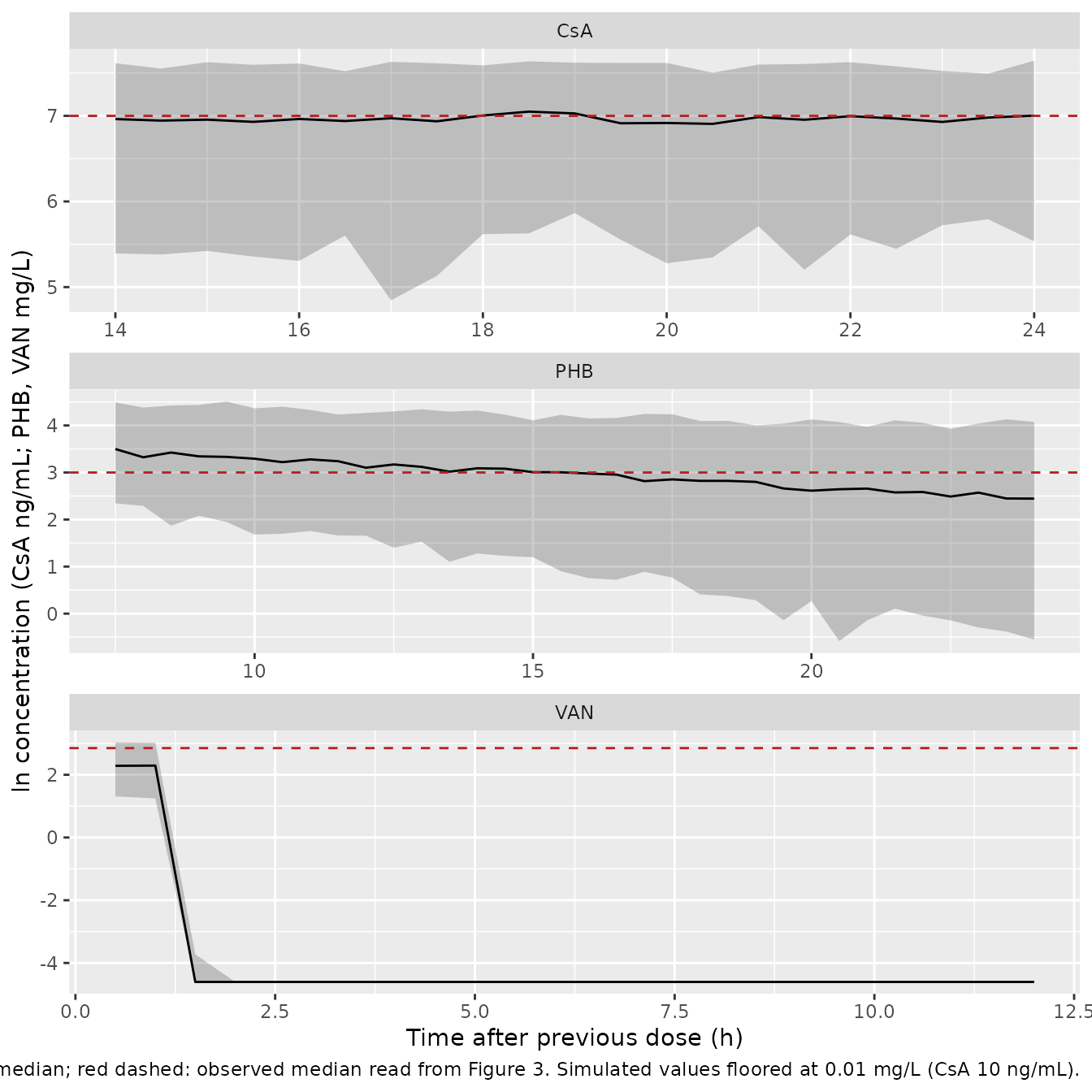
Back 2019 does not report individual doses, so the regimens below are assumptions (listed under Assumptions and deviations). Figure 3 plots the natural log of concentration against time after the previous dose; the observed medians read from it are about ln 7.0 for CsA (1100 ng/mL), ln 3.0 for PHB (20 mg/L) and ln 2.85 for VAN (17 mg/L). The y-axis unit labels of Figure 3a (ug/mL) and Figure 3c (ng/mL) are swapped relative to these magnitudes.

# set.seed() seeds R's covariate draws only. rxode2's simulation RNG is
# partitioned per solver thread, so the simulated cohort differs between
# machines with different thread counts; every assertion below is written to
# hold for any cohort.
set.seed(2019)
rxode2::rxSetSeed(2019)
n_arm <- 200L

rtrunc_norm <- function(n, mean, sd, lo, hi) {
  x <- rnorm(n, mean, sd)
  while (any(bad <- x < lo | x > hi)) x[bad] <- rnorm(sum(bad), mean, sd)
  x
}
# Weight and PCA as a Gaussian copula (correlation assumed 0.8), each margin
# log-normal with the Table 1 mean and SD, truncated to the Table 1 range.
copula_cov <- function(n, m_wt, s_wt, r_wt, m_pa, s_pa, r_pa, rho = 0.8) {
  out <- matrix(NA_real_, 0, 2)
  sl <- function(m, s) sqrt(log(1 + (s / m)^2))
  while (nrow(out) < n) {
    z1 <- rnorm(n)
    z2 <- rho * z1 + sqrt(1 - rho^2) * rnorm(n)
    wt <- m_wt * exp(sl(m_wt, s_wt) * z1 - sl(m_wt, s_wt)^2 / 2)
    pa <- m_pa * exp(sl(m_pa, s_pa) * z2 - sl(m_pa, s_pa)^2 / 2)
    ok <- wt >= r_wt[1] & wt <= r_wt[2] & pa >= r_pa[1] & pa <= r_pa[2]
    out <- rbind(out, cbind(wt[ok], pa[ok]))
  }
  out[seq_len(n), , drop = FALSE]
}

cov_csa <- data.frame(id = seq_len(n_arm), WT = rtrunc_norm(n_arm, 12.9, 3.8, 5, 24), PAGE = 40)
m_phb <- copula_cov(n_arm, 3.3, 1, c(1, 6.9), 41.3, 3.9, c(31, 51.1))
cov_phb <- data.frame(id = seq_len(n_arm), WT = m_phb[, 1], PAGE = m_phb[, 2])
m_van <- copula_cov(n_arm, 3.2, 2.6, c(0.4, 14.9), 41.2, 14.2, c(25.6, 110))
cov_van <- data.frame(id = seq_len(n_arm), WT = m_van[, 1], PAGE = m_van[, 2])

# CsA: two consecutive 24-h infusions (days 1 and 2); observe 14-24 h after
# the start of the day-2 infusion (Figure 3a window).
ev_csa <- dplyr::bind_rows(
  cov_csa |> tidyr::crossing(time = c(0, 24)) |>
    dplyr::mutate(evid = 1, amt = 12 * WT, dur = 24, cmt = "central"),
  cov_csa |> tidyr::crossing(time = 24 + seq(14, 24, by = 0.5)) |>
    dplyr::mutate(evid = 0, amt = 0, dur = 0, cmt = "central")
) |> dplyr::arrange(id, time, dplyr::desc(evid))

# PHB: 20 mg/kg IV loading over 30 min, then 4 mg/kg oral every 24 h from
# 24 h; observe 7.5-25 h after the seventh maintenance dose (Figure 3b).
ev_phb <- dplyr::bind_rows(
  cov_phb |> dplyr::mutate(time = 0, evid = 1, amt = 20 * WT, dur = 0.5, cmt = "central"),
  cov_phb |> tidyr::crossing(time = 24 * (1:7)) |>
    dplyr::mutate(evid = 1, amt = 4 * WT, dur = 0, cmt = "depot"),
  cov_phb |> tidyr::crossing(time = 168 + seq(7.5, 24, by = 0.5)) |>
    dplyr::mutate(evid = 0, amt = 0, dur = 0, cmt = "central")
) |> dplyr::arrange(id, time, dplyr::desc(evid))

# VAN: 15 mg/kg over 1 h every 12 h for 3 days; observe 0.5-12 h after the
# sixth dose (Figure 3c).
ev_van <- dplyr::bind_rows(
  cov_van |> tidyr::crossing(time = 12 * (0:5)) |>
    dplyr::mutate(evid = 1, amt = 15 * WT, dur = 1, cmt = "central"),
  cov_van |> tidyr::crossing(time = 60 + seq(0.5, 12, by = 0.5)) |>
    dplyr::mutate(evid = 0, amt = 0, dur = 0, cmt = "central")
) |> dplyr::arrange(id, time, dplyr::desc(evid))

sim_vpc <- function(drug, ev, t_prev) {
  rxode2::rxSolve(ui[[drug]], events = ev, keep = c("WT", "PAGE")) |>
    as.data.frame() |>
    dplyr::mutate(drug = drug, tad = time - t_prev)
}
vpc <- dplyr::bind_rows(
  sim_vpc("CsA", ev_csa, 24),
  sim_vpc("PHB", ev_phb, 168),
  sim_vpc("VAN", ev_van, 60)
)
stopifnot(all(c("sim", "Cc") %in% names(vpc)), !anyNA(vpc$Cc))

# Simulated observations are floored at 0.01 mg/L (10 ng/mL for CsA) before
# the log: proportional error can draw non-positive values, and the printed
# vancomycin parameters drive concentrations down to integrator noise, whose
# logarithm is meaningless.
floor_conc <- c(CsA = 10, PHB = 0.01, VAN = 0.01)
vpc_q <- vpc |>
  dplyr::mutate(lsim = log(pmax(sim, floor_conc[drug]))) |>
  dplyr::group_by(drug, tad) |>
  dplyr::summarise(
    q05 = quantile(lsim, 0.05), q50 = quantile(lsim, 0.50),
    q95 = quantile(lsim, 0.95), .groups = "drop"
  )
pct_floor_van <- 100 * mean(vpc$sim[vpc$drug == "VAN"] < floor_conc[["VAN"]])
observed_median <- data.frame(drug = c("CsA", "PHB", "VAN"), ln_obs = c(7.0, 3.0, 2.85))

ggplot(vpc_q, aes(tad, q50)) +
  geom_ribbon(aes(ymin = q05, ymax = q95), alpha = 0.25) +
  geom_line() +
  geom_hline(data = observed_median, aes(yintercept = ln_obs), linetype = "dashed", colour = "firebrick") +
  facet_wrap(~drug, ncol = 1, scales = "free") +
  labs(
    x = "Time after previous dose (h)",
    y = "ln concentration (CsA ng/mL; PHB, VAN mg/L)",
    caption = paste(
      "Replicates Figure 3 of Back 2019 under assumed regimens.",
      "Grey: simulated 5th-95th percentile; line: median; red dashed: observed median read from Figure 3.",
      "Simulated values floored at 0.01 mg/L (CsA 10 ng/mL)."
    )
  )

vpc_sum <- vpc_q |>
  dplyr::group_by(drug) |>
  dplyr::summarise(
    sim_median = median(q50),
    upper_half = median(q95 - q50),
    fall = q50[which.min(tad)] - q50[which.max(tad)],
    .groups = "drop"
  ) |>
  dplyr::left_join(observed_median, by = "drug")
knitr::kable(
  vpc_sum |>
    dplyr::rename("Drug" = drug, "Simulated median (ln)" = sim_median,
                  "Simulated 95th minus median (ln)" = upper_half,
                  "Fall across window (ln)" = fall, "Observed median (ln)" = ln_obs),
  digits = 2,
  caption = "Simulated VPC summaries against the observed medians of Figure 3."
)

Simulated VPC summaries against the observed medians of Figure 3.

Drug	Simulated median (ln)	Simulated 95th minus median (ln)	Fall across window (ln)	Observed median (ln)
CsA	6.96	0.63	-0.04	7.00
PHB	2.99	1.22	1.05	3.00
VAN	-4.61	0.00	6.89	2.85

csa <- vpc_sum[vpc_sum$drug == "CsA", ]
van <- vpc_sum[vpc_sum$drug == "VAN", ]
phb <- vpc_sum[vpc_sum$drug == "PHB", ]
stopifnot(
  # CsA reproduces: the median lands near Figure 3a under the assumed dose,
  # and the upper half-band of IIV plus 46.8% proportional error (expected
  # 0.65 ln units; 0.28 if propSd were ten times smaller, 2.2 if ten times
  # larger) matches the Figure 3a 95th-percentile line, about 0.5-0.7 above
  # the median. The lower half is not used: the floor truncates it.
  abs(csa$sim_median - 7.0) < 0.5,
  csa$upper_half > 0.45, csa$upper_half < 0.9,
  # Known deviation, VAN: the printed CL/Vd put the simulated median several
  # log units below the observed median at any plausible neonatal dose.
  van$sim_median < van$ln_obs - 2,
  pct_floor_van > 50,
  # Known deviation, PHB: the printed Vd makes the profile fall steeply over a
  # window in which Figure 3b is flat.
  phb$fall > 0.5
)

The CsA model reproduces its own VPC. The phenobarbital simulated median sits near the observed level, but the profile falls steeply across the dosing interval where Figure 3b is flat, and its plotted 5th-95th band is much wider than the observed one (about ln 2.1 to 3.9). For vancomycin, 91% of the simulated observations 0.5-12 h after the dose are below 0.01 mg/L, so the median sits on the display floor while the observed median is about 17 mg/L. Both phenobarbital and vancomycin are known deviations of the published parameter values, recorded in the gate so that a change to them is noticed. They are not failures of the encoding.

Errata

Back 2019 has no supplementary material and no NONMEM control stream. No correction had been registered as of 2026-10-16 (Crossref update-to and updated-by empty, Europe PMC commentCorrectionList empty, no PubMed correction link). Table 3 is internally consistent, because every bootstrap interval brackets its point estimate. The disagreement is between Table 3 and the paper’s own Figure 3. The maintainers encoded Table 3 verbatim and did not correct either parameter set.

• Phenobarbital Vd. CL reproduces the observed level: at the stated 3-5 mg/kg/day maintenance dose and F = 0.724, the typical-subject average steady-state concentration is about 18-30 mg/L, against an observed median of about 20 mg/L. However, Vd = 5.51 L at 70 kg is 0.08 L/kg and gives an 11-h half-life in the typical neonate. That implies a fall of about two thirds over the 7.5-25 h window, where the Figure 3b median is flat. A flat window needs Vd of at least about 58 L at 70 kg, roughly ten times the printed value, which is consistent with a decimal slip (55.1 printed as 5.51). This is an inference and has not been applied.
• Vancomycin CL and Vd. The printed values give a typical-neonate CL of 1.47 L/h/kg, a Vd of 0.046 L/kg and a half-life of 1.3 minutes. The paper samples 0.5-23.5 h after the dose, which would be more than 20 half-lives, yet Figure 3c shows measurable concentrations across that whole window. The chunk below shows that swapping the CL and Vd rows of Table 3 (CL 3.23 L/h and Vd 69.4 L at 70 kg) gives a typical neonate with CL 0.07 L/h/kg, Vd 1.0 L/kg and a 10-h half-life. At 15 mg/kg every 12 h, that predicts an average concentration close to the observed 17 mg/L. This is shown for information only: the swap is a hypothesis about a table-layout error and is not applied to the model.
• Reading Table 3 as values at the cohort’s typical weight rather than at 70 kg does not rescue the set. It fixes the vancomycin Vd but makes the phenobarbital and vancomycin CL tens to hundreds of times too high.

van_t <- typ[typ$drug == "VAN", ]
swap <- tibble::tibble(
  reading = c("Table 3 as printed (encoded)", "CL and Vd rows swapped (not applied)"),
  tvcl = c(69.4, 3.23),
  tvv = c(3.23, 69.4)
) |>
  dplyr::mutate(
    cl = tvcl * (van_t$WT / 70)^0.75 * van_t$fmat,
    v = tvv * (van_t$WT / 70),
    thalf_h = log(2) * v / cl,
    cavg_15q12 = 30 * van_t$WT / 24 / cl
  )
knitr::kable(
  swap |>
    dplyr::select(reading, cl, v, thalf_h, cavg_15q12) |>
    dplyr::rename("Reading" = reading, "CL (L/h)" = cl, "Vd (L)" = v,
                  "t1/2 (h)" = thalf_h, "Cavg,ss at 15 mg/kg q12h (mg/L)" = cavg_15q12),
  digits = 3,
  caption = "Typical vancomycin neonate (3.2 kg, PCA 41.2 weeks); observed median about 17 mg/L."
)

Typical vancomycin neonate (3.2 kg, PCA 41.2 weeks); observed median about 17 mg/L.

Reading	CL (L/h)	Vd (L)	t1/2 (h)	Cavg,ss at 15 mg/kg q12h (mg/L)
Table 3 as printed (encoded)	4.710	0.148	0.022	0.849
CL and Vd rows swapped (not applied)	0.219	3.173	10.033	18.249

Assumptions and deviations

• Doses. No individual doses are reported. The regimens behind Figure 3 are assumptions. The CsA rate of 12 mg/kg per 24 h was back-calculated by the maintainers so that the typical subject sits at the Figure 3a median; the paper says only “high dose”. PHB uses 20 mg/kg IV loading and 4 mg/kg/day oral, the midpoints of the stated ranges. VAN uses 15 mg/kg over 1 h every 12 h, inside the stated 6-24 h interval range. Only the CsA spread and the shape and level contrasts of PHB and VAN are interpreted.
• Covariates. Weight and post-conceptional age are drawn as log-normal margins with the Table 1 mean and SD, truncated to the Table 1 range, joined by an assumed correlation of 0.8; the paper reports no joint distribution. CsA has no maturation function, so its cohort carries a placeholder PAGE = 40 that the model does not use.
• Age variable. Eq 8 writes the maturation driver as “Age”; Methods Eq 2 and Eq 5 define it as post-conceptional age, consistent with TM50 in weeks. It is supplied as PAGE in weeks.
• Allometric exponents. The Discussion says estimated exponents fit the infant datasets better than 0.75, but no estimated exponent is tabulated, and Eq 7 and Eq 8 print 1 and 0.75. The printed equations govern.
• TM50 and Hill. Results 3.3 says both were applied from reference values (ref 2, Holford 2013). Table 3 marks only the vancomycin pair as held constant; the phenobarbital pair carries RSEs and bootstrap intervals and is encoded as estimated.
• IIV. Table 3 reports IIV as CV%. The variances use omega^2 = log(CV^2 + 1). No IIV covariances are reported, and nothing printed (no interval on the IIV terms) separates this reading from CV = 100 * sqrt(omega). The two readings differ in variance by under 2% for both CsA terms and the vancomycin CL, by 8% for the phenobarbital CL, 13% for the vancomycin Vd and 28% for the phenobarbital Vd (0.482 here against 0.619).
• Residual error. Concentrations were log-transformed before fitting, and Eq 6 writes the constant-CV model as C = Cpred * (1 + eps). The model encodes that printed proportional form. For the VPC, simulated observations are floored at 0.01 mg/L (10 ng/mL for CsA) before taking logs.
• Units and specimen. CsA is returned in ng/mL (doses in mg, volumes in L, multiplied by 1000), matching the magnitude of Figure 3a; PHB and VAN are returned in mg/L. The Methods call the samples “blood”; Figure 3 labels them plasma, and the model files record plasma.