Paracetamol (Krekels 2015) • nlmixr2lib

Model and source

Citation: Krekels EHJ, van Ham S, Allegaert K, de Hoon J, Tibboel D, Danhof M, Knibbe CAJ (2015). Developmental changes rather than repeated administration drive paracetamol glucuronidation in neonates and infants. European Journal of Clinical Pharmacology 71(9):1075-1082. doi:10.1007/s00228-015-1887-y.
Description: Parent-and-metabolites population PK model for intravenous paracetamol (administered as the prodrug propacetamol; doses expressed as paracetamol equivalents) and its glucuronide and sulphate phase-II conjugates in 54 preterm and term neonates and infants (Krekels 2015). One-compartment plasma disposition for paracetamol with three parallel elimination pathways from the central compartment: glucuronide formation (CL_gluc), sulphate formation (CL_sulf), and unchanged renal excretion (CL_renal). Each metabolite distributes into a one-compartment plasma space whose volume is fixed at 18% of the parent volume (Vc_gluc = Vc_sulf = 0.18 * Vc, based on the previously reported adult paracetamol model in Allegaert et al. and adult literature). The two metabolites share a common urinary excretion rate constant kE_met = mf * kE_renal, where kE_renal = CL_renal / Vc is the parent unchanged-renal rate constant and mf (multiplication factor) is estimated to be 11.3. Cumulative urinary amounts of parent paracetamol and the two metabolites are tracked as elimination-amount compartments and exposed as additive-error observations. Bodyweight enters linearly on Vc (and so on the metabolite volumes by inheritance), on the glucuronide formation clearance (CL_gluc), and on the unchanged renal clearance (CL_renal); the sulphate formation clearance (CL_sulf) scales with bodyweight as a power with an estimated exponent of 1.40. No postnatal age, postmenstrual age, sex, term-vs-preterm, or study-protocol covariate was retained in the final model, and no time-varying (up-regulation) component was detected on the glucuronidation pathway. Parameter values reported throughout (mL/min/kg, L/kg) are per-kg quantities; individual structural parameters are obtained in model() by multiplying by body weight in kg (linear) or body weight in kg raised to n (power).
Article: https://doi.org/10.1007/s00228-015-1887-y

The paper develops a one-compartment parent-and-two-metabolite popPK model for intravenous paracetamol (administered as propacetamol, doses expressed as paracetamol equivalents) in preterm and term neonates and infants. Pooled plasma paracetamol concentrations and urinary recoveries of unchanged paracetamol, paracetamol-glucuronide, and paracetamol-sulphate were used. The model serves to test whether glucuronidation upregulates after repeated dosing; the authors conclude that bodyweight-driven developmental changes alone explain the observed time trends and that no time-varying (up-regulation) component is needed.

Population

Krekels 2015 pools two clinical studies (one single-dose, one multiple-dose) carried out at University Hospital Leuven (Belgium) and Erasmus MC-Sophia Children’s Hospital (Rotterdam, Netherlands). The final dataset comprises 54 preterm and term neonates and young infants with a median bodyweight of 2.5 kg (range 0.5-6.3 kg), median postnatal age of 1 day (range 1-140 days), and median postmenstrual age of 36 weeks (range 27-60 weeks). Paracetamol plasma concentrations were available from all 54 subjects (353 observations); urine collections in 6, 8, or 12 h aliquots were available for 22 of the 54 subjects (435 observations of unchanged paracetamol or one of the two metabolites).

The same population information is available programmatically:

local({
  fbody <- body(readModelDb("Krekels_2015_paracetamol"))
  meta_env <- new.env()
  for (stmt in as.list(fbody)[-1]) {
    if (is.call(stmt) && length(stmt) >= 1 &&
        identical(stmt[[1]], as.name("<-"))) {
      eval(stmt, envir = meta_env)
    } else {
      break
    }
  }
  cat("Population:\n")
  str(meta_env$population, max.level = 1)
  cat("\nCovariates:\n")
  str(meta_env$covariateData, max.level = 1)
})
#> Population:
#> List of 13
#>  $ species       : chr "human"
#>  $ n_subjects    : int 54
#>  $ n_studies     : int 2
#>  $ age_range     : chr "PNA 1-140 days; PMA 27-60 weeks"
#>  $ age_median    : chr "PNA 1 day; PMA 36 weeks"
#>  $ weight_range  : chr "0.5-6.3 kg"
#>  $ weight_median : chr "2.5 kg"
#>  $ sex_female_pct: num NA
#>  $ race_ethnicity: chr NA
#>  $ disease_state : chr "Preterm and term neonates and young infants admitted to the neonatal intensive care unit (NICU). Paracetamol wa"| __truncated__
#>  $ dose_range    : chr "Single-dose study: 20 or 40 mg/kg propacetamol (paracetamol equivalent 10 or 20 mg/kg) on the first day of post"| __truncated__
#>  $ regions       : chr "Belgium (Leuven), Netherlands (Rotterdam)"
#>  $ notes         : chr "Two studies pooled: a single-dose study (plasma sampling up to 10 h post-dose) and a repeated-dose study with u"| __truncated__
#> 
#> Covariates:
#> List of 1
#>  $ WT:List of 6

Source trace

Per-parameter and per-equation origin (also recorded as in-file comments in inst/modeldb/specificDrugs/Krekels_2015_paracetamol.R):

Equation / parameter	Value (typical, per kg)	Source location
`lvc`	`log(1.06)` L/kg	Table 1: V1 (RSE 4.34%)
`lcl_gluc`	`log(0.266)` mL/min/kg	Table 1: CL1 (RSE 17.4%)
`lcl_sulf`	`log(1.46)` mL/min/kg^n	Table 1: CL2 (RSE 14.8%)
`lcl_renal`	`log(0.285)` mL/min/kg	Table 1: CL4 (RSE 6.98%)
`e_wt_cl_sulf`	`1.40`	Table 1: n (RSE 9.29%)
`lmf`	`log(11.3)`	Table 1: mf (RSE 21.5%)
`frac_vmet`	`0.18 FIX`	Methods: V2 = V3 = 0.18*V1, fixed from adult data (refs 13-14)
`etalvc`	`~ 0.0925`	Table 1: IIV V1 (RSE 29.5%)
`etalcl_gluc`	`~ 0.599`	Table 1: IIV CL1 (RSE 41.6%)
`etalcl_sulf`	`~ 0.312`	Table 1: IIV CL2 (RSE 33.3%)
`etalcl_renal`	`~ 0.0879`	Table 1: IIV CL4 (RSE 52.2%)
`addSd`	`sqrt(0.354)` mg/L	Table 1: P plasma additive variance (RSE 29.4%)
`propSd`	`sqrt(0.0198)`	Table 1: P plasma proportional variance (RSE 16.5%)
`addSd_urineP`	`sqrt(0.188)` mg	Table 1: P urine additive variance (RSE 27.5%)
`addSd_urinePG`	`sqrt(0.223)` mg	Table 1: PG urine additive variance (RSE 14.5%)
`addSd_urinePS`	`sqrt(0.332)` mg	Table 1: PS urine additive variance (RSE 35.9%)
`d/dt(central)` ODE	n/a	Figure 1 schematic
`d/dt(central_gluc)` ODE	n/a	Figure 1 schematic
`d/dt(central_sulf)` ODE	n/a	Figure 1 schematic
`d/dt(urine)` ODE	n/a	Figure 1 schematic
`d/dt(urine_gluc)` ODE	n/a	Figure 1 schematic
`d/dt(urine_sulf)` ODE	n/a	Figure 1 schematic
Linear bodyweight covariate (Vc, CL_gluc, CL_renal)	n/a	Results: linear BW relationships
Power bodyweight covariate (CL_sulf)	`WT^n`, n = 1.40	Results: exponential equation with estimated n

Virtual cohort

The Krekels 2015 simulation in Figure 3 uses a single ‘typical individual’ with bodyweight 2.5 kg (the median of the cohort) receiving a single 15 mg/kg paracetamol-equivalent dose as a 15-minute IV infusion. We reproduce that scenario directly here and additionally build a small stochastic VPC across the published bodyweight range (0.5-6.3 kg) to illustrate inter-individual variability.

set.seed(2026L)

dose_mg_per_kg <- 15      # paracetamol-equivalent loading dose
inf_dur_min    <- 15      # 15-minute infusion
horizon_min    <- 36 * 60 # follow-up window (36 h)
times_obs      <- sort(unique(c(seq(0, horizon_min, by = 30),
                                c(6, 12, 18, 24, 30, 36) * 60)))

make_cohort <- function(wt, n = 1L, id_offset = 0L) {
  # wt: vector of body weights (kg); n: number of subjects per weight.
  tibble(
    id = id_offset + seq_len(length(wt) * n),
    WT = rep(wt, each = n)
  ) |>
    mutate(amt_mg = dose_mg_per_kg * WT,
           rate_mg_per_min = amt_mg / inf_dur_min)
}

# Typical 2.5 kg infant (Krekels 2015 Figure 3 'typical individual').
typical <- make_cohort(wt = 2.5, n = 1L)

# Stochastic cohort spanning the published weight range.
vpc_cohort <- make_cohort(wt = round(seq(0.5, 6.3, length.out = 12), 2),
                          n = 5L, id_offset = 10L)

build_events <- function(cohort) {
  doses <- cohort |>
    transmute(id, time = 0, evid = 1L, amt = amt_mg,
              rate = rate_mg_per_min, cmt = "central", WT = WT)
  obs <- cohort |>
    tidyr::expand_grid(time = times_obs) |>
    transmute(id, time, evid = 0L, amt = NA_real_, rate = NA_real_,
              cmt = "Cc", WT = WT)
  bind_rows(doses, obs) |>
    arrange(id, time, desc(evid))
}

events_typ <- build_events(typical)
events_vpc <- build_events(vpc_cohort)

stopifnot(!anyDuplicated(unique(events_typ[, c("id", "time", "evid")])))
stopifnot(!anyDuplicated(unique(events_vpc[, c("id", "time", "evid")])))

Simulation

Two simulations are produced. The first is the Figure 3 ‘typical individual’ (typical-value parameters via rxode2::zeroRe(), 2.5 kg infant, single 15 mg/kg dose). The second is a stochastic VPC across the published weight range; we keep IIV non-zero so the spread reflects the model’s between-subject variability for V_c, CL_gluc, CL_sulf, and CL_renal.

mod_full    <- readModelDb("Krekels_2015_paracetamol")
mod_typical <- rxode2::zeroRe(mod_full)
#> ℹ parameter labels from comments will be replaced by 'label()'

sim_typ <- rxode2::rxSolve(mod_typical, events = events_typ,
                           keep = c("WT")) |>
  as.data.frame() |>
  dplyr::mutate(id = 1L) |>
  dplyr::filter(time >= 0)
#> ℹ omega/sigma items treated as zero: 'etalvc', 'etalcl_gluc', 'etalcl_sulf', 'etalcl_renal'

sim_vpc <- rxode2::rxSolve(mod_full, events = events_vpc,
                           keep = c("WT")) |>
  as.data.frame() |>
  dplyr::filter(time >= 0)
#> ℹ parameter labels from comments will be replaced by 'label()'

Replicate Figure 3 (cumulative urinary recovery)

Krekels 2015 Figure 3 plots the relative cumulative amount of unchanged paracetamol (P), paracetamol-glucuronide (PG), and paracetamol-sulphate (PS) recovered in urine over 36 hours after a single 15 mg/kg paracetamol-equivalent dose in a typical 2.5 kg individual. The recoveries are expressed as molar paracetamol equivalents normalised to the administered dose (i.e. percent of dose).

dose_typ_mg <- typical$amt_mg

fig3 <- sim_typ |>
  transmute(
    time_h    = time / 60,
    P_pct     = 100 * urineP  / dose_typ_mg,
    PG_pct    = 100 * urinePG / dose_typ_mg,
    PS_pct    = 100 * urinePS / dose_typ_mg
  ) |>
  tidyr::pivot_longer(c(P_pct, PG_pct, PS_pct),
                      names_to = "species", values_to = "pct_dose") |>
  dplyr::mutate(species = factor(species,
                                 levels = c("PS_pct", "PG_pct", "P_pct"),
                                 labels = c("Paracetamol-sulphate (PS)",
                                            "Paracetamol-glucuronide (PG)",
                                            "Unchanged paracetamol (P)")))

ggplot(fig3, aes(time_h, pct_dose, colour = species)) +
  geom_line(linewidth = 0.8) +
  scale_x_continuous(breaks = seq(0, 36, by = 6)) +
  labs(
    x = "Time after dose (h)",
    y = "Cumulative urinary recovery (% of administered dose)",
    colour = NULL,
    title = paste(
      "Replicates Figure 3 of Krekels 2015:",
      "relative cumulative urinary recovery of P, PG, PS"
    ),
    caption = "Typical 2.5 kg individual, single 15 mg/kg paracetamol-equivalent IV infusion over 15 minutes."
  ) +
  theme_minimal()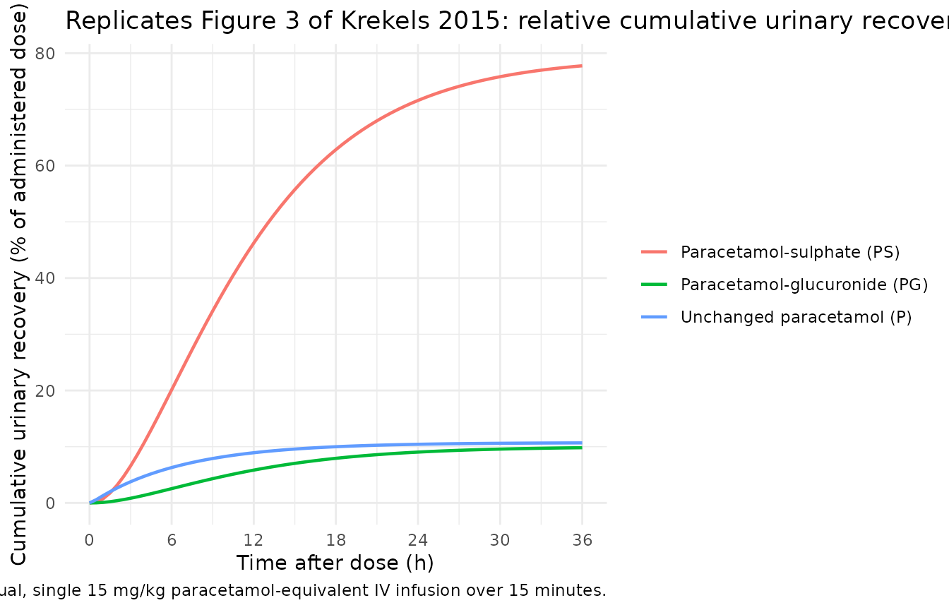

The per-6-h-interval fractions of dose recovered as each species can be read off the cumulative trajectory by differencing successive 6-hour values. Krekels 2015 Figure 3 annotates these percentages across the top of the panel; we tabulate them here.

interval_table <- sim_typ |>
  dplyr::filter(time %in% (c(6, 12, 18, 24, 30, 36) * 60)) |>
  dplyr::transmute(
    interval_h_end = time / 60,
    P_mg     = urineP,
    PG_mg    = urinePG,
    PS_mg    = urinePS
  ) |>
  dplyr::arrange(interval_h_end) |>
  dplyr::mutate(
    P_in_interval_pct  = 100 * (P_mg  - dplyr::lag(P_mg,  default = 0)) / dose_typ_mg,
    PG_in_interval_pct = 100 * (PG_mg - dplyr::lag(PG_mg, default = 0)) / dose_typ_mg,
    PS_in_interval_pct = 100 * (PS_mg - dplyr::lag(PS_mg, default = 0)) / dose_typ_mg
  ) |>
  dplyr::transmute(
    interval     = paste0(interval_h_end - 6, "-", interval_h_end, " h"),
    P_pct        = round(P_in_interval_pct,  2),
    PG_pct       = round(PG_in_interval_pct, 2),
    PS_pct       = round(PS_in_interval_pct, 2),
    total_pct    = round(P_in_interval_pct + PG_in_interval_pct +
                         PS_in_interval_pct, 2)
  )

knitr::kable(
  interval_table,
  caption = paste(
    "Percentage of administered dose recovered as unchanged paracetamol (P),",
    "paracetamol-glucuronide (PG), and paracetamol-sulphate (PS) in each",
    "6-h urine collection interval, typical 2.5 kg infant."
  )
)

Percentage of administered dose recovered as unchanged paracetamol (P), paracetamol-glucuronide (PG), and paracetamol-sulphate (PS) in each 6-h urine collection interval, typical 2.5 kg infant.
interval	P_pct	PG_pct	PS_pct	total_pct
0-6 h	6.29	2.54	20.11	28.94
6-12 h	2.63	3.30	26.11	32.05
12-18 h	1.07	2.10	16.61	19.78
18-24 h	0.43	1.11	8.75	10.29
24-30 h	0.18	0.53	4.22	4.93
30-36 h	0.07	0.24	1.94	2.26

The sulphate pathway dominates in this very young population, with glucuronide the next-largest fraction; unchanged renal excretion is small. As Krekels 2015 discusses, the glucuronide fraction increases over time relative to the sulphate fraction not because of up-regulation of UGT activity but simply because the glucuronide formation clearance is slower, so the metabolite appears later in the urine.

VPC of plasma paracetamol across the published weight range

This figure overlays per-subject plasma paracetamol profiles for 12 weights spanning 0.5-6.3 kg with 5 stochastic subjects per weight. The 5th, 50th, and 95th simulated-population percentiles are overlaid as ribbons.

vpc_quantiles <- sim_vpc |>
  dplyr::group_by(time) |>
  dplyr::summarise(
    Q05 = quantile(Cc, 0.05, na.rm = TRUE),
    Q50 = quantile(Cc, 0.50, na.rm = TRUE),
    Q95 = quantile(Cc, 0.95, na.rm = TRUE),
    .groups = "drop"
  )

ggplot(vpc_quantiles, aes(x = time / 60)) +
  geom_ribbon(aes(ymin = Q05, ymax = Q95), alpha = 0.25) +
  geom_line(aes(y = Q50), linewidth = 0.7) +
  scale_y_log10() +
  scale_x_continuous(breaks = seq(0, 36, by = 6)) +
  labs(
    x = "Time after dose (h)",
    y = "Plasma paracetamol Cc (mg/L, log scale)",
    title = "Stochastic VPC of plasma paracetamol (60 subjects spanning 0.5-6.3 kg)",
    caption = "Median (line) and 5th-95th percentiles (ribbon) of simulated plasma Cc."
  ) +
  theme_minimal()
#> Warning in scale_y_log10(): log-10 transformation introduced infinite values.
#> log-10 transformation introduced infinite values.
#> log-10 transformation introduced infinite values.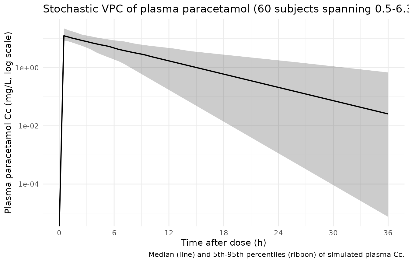

PKNCA validation on plasma paracetamol

PKNCA non-compartmental analysis is run on the typical-value plasma trajectory (2.5 kg, single 15 mg/kg dose). With only one subject and a single dose level there is no meaningful between-cohort comparison; the goal here is to show that Cmax, AUC, and half-life align with the expected typical-individual values.

sim_nca <- sim_typ |>
  dplyr::filter(!is.na(Cc), Cc > 0, time > 0) |>
  dplyr::transmute(id, time_h = time / 60, Cc, cohort = "typical_2.5kg")

conc_obj <- PKNCA::PKNCAconc(sim_nca, Cc ~ time_h | cohort + id)

dose_df <- events_typ |>
  dplyr::filter(evid == 1L) |>
  dplyr::transmute(id, time_h = time / 60, amt, cohort = "typical_2.5kg")

dose_obj <- PKNCA::PKNCAdose(dose_df, amt ~ time_h | cohort + id)

intervals <- data.frame(
  start      = 0,
  end        = Inf,
  cmax       = TRUE,
  tmax       = TRUE,
  aucinf.obs = TRUE,
  half.life  = TRUE
)

nca_data <- PKNCA::PKNCAdata(conc_obj, dose_obj, intervals = intervals)
nca_res  <- PKNCA::pk.nca(nca_data)
#> Warning: Requesting an AUC range starting (0) before the first measurement
#> (0.5) is not allowed

knitr::kable(
  as.data.frame(nca_res$result) |>
    dplyr::filter(PPTESTCD %in% c("cmax", "tmax", "aucinf.obs", "half.life")) |>
    dplyr::transmute(
      cohort,
      parameter = PPTESTCD,
      value     = signif(PPORRES, 4)
    ) |>
    tidyr::pivot_wider(names_from = parameter, values_from = value),
  caption = paste(
    "Typical-value PKNCA on simulated plasma paracetamol after a single",
    "15 mg/kg paracetamol-equivalent IV (15 min infusion) in a 2.5 kg",
    "infant. Units: Cmax in mg/L, Tmax / half-life in h, AUC[0-Inf] in",
    "mg*h/L."
  )
)

Typical-value PKNCA on simulated plasma paracetamol after a single 15 mg/kg paracetamol-equivalent IV (15 min infusion) in a 2.5 kg infant. Units: Cmax in mg/L, Tmax / half-life in h, AUC[0-Inf] in mg*h/L.
cohort	cmax	tmax	half.life	aucinf.obs
typical_2.5kg	13.38	0.5	4.608	NA

Comparison against published NCA

Krekels 2015 does not report NCA Cmax / AUC / half-life as a separate results table; its primary outputs are the structural model parameter estimates (Table 1) and the Figure 3 cumulative urinary recovery panel. The Cmax and half-life from the PKNCA call above can be sanity-checked against the structural model: V_c at 2.5 kg is 1.06 * 2.5 = 2.65 L, so a 37.5 mg paracetamol-equivalent dose delivered as a 15-minute infusion gives an expected end-of-infusion concentration on the order of 13 mg/L (with infusion-time distribution lowering the peak slightly from the instantaneous-bolus 37.5 / 2.65 ~= 14.2 mg/L). The total elimination rate at 2.5 kg is CL_gluc/V_c + CL_sulf/V_c + CL_renal/V_c = (0.266 + 1.46 * 2.5^0.40 + 0.285) * 2.5 / 2650 ~= 0.0025 1/min, implying a half-life of ~4.7 h, consistent with the published neonatal paracetamol literature.

Assumptions and deviations

Metabolite volume rule. V_gluc and V_sulf are fixed at 0.18 * V_central per Krekels 2015 Methods, citing Anderson et al. (ref 13) and Critchley et al. (ref 14). The model file declares frac_vmet <- fixed(0.18) to preserve this provenance.
Shared metabolite urinary-excretion rate constant. Krekels 2015 assumes k3 = k5 = mf * k4 with one common multiplication factor mf = 11.3 estimated for both glucuronide and sulphate, so the model file derives both metabolite urinary-excretion rate constants from the single mf parameter.
Per-kg parameterization. Table 1 reports each structural parameter in per-kg units (L/kg or mL/min/kg, with the sulphate formation clearance carrying an estimated power exponent of 1.40). The model file’s ini() entries therefore represent the typical parameter at WT = 1 kg, with linear or power bodyweight scaling applied inside model().
CL_sulf bodyweight exponent. Krekels 2015 calls this an ‘exponential’ covariate equation; in their notation, P_i = P_p * cov^n with n estimated. This is structurally a power function (not literally an exponential of bodyweight) and the model file implements it as (WT/wt_ref)^e_wt_cl_sulf.
NONMEM variance -> nlmixr2 SD. Table 1 reports the variance of each residual-error component (and of each IIV eta). The IIV values are used directly because the eta is log-normal with omega^2 as the internal variance scale; the residual-error values are square-rooted in ini() because nlmixr2’s add(...) and prop(...) arguments are standard deviations rather than variances.
Compartment-naming warnings. The three urine compartments (urine, urine_gluc, urine_sulf) and the observation variables (urineP, urinePG, urinePS) follow the same cumulative-elimination idiom used by Pierre_2017_morphine.R (urine_morphine, urine_m3g) and Allegaert_2015_paracetamol.R (urine_apap, urine_gluc, urine_sulf). urine is not in R/conventions.R’s canonical compartment list, so checkModelConventions() emits warnings for these names; the convention here is consistent with the existing models for the same biological concept (cumulative urinary recovery of parent and metabolites).
Dose units. The model expects paracetamol-equivalent mg as the dose. Datasets that record propacetamol mg should convert to paracetamol equivalents on a molar basis (paracetamol MW 151.16 vs propacetamol MW 264.27) before dosing.
Observation-time differencing for urine amounts. Krekels 2015 fit per-collection-interval urine amounts; the model exposes cumulative-urine compartments and observation variables. Downstream users who want per-interval recoveries (as in the table replicated above) should difference the cumulative output between successive collection-interval endpoints.
Covariates not retained. Postnatal age, postmenstrual age, sex, term-vs-preterm-birth, and the source-study indicator were tested but were not retained in the final Krekels 2015 model; bodyweight was the only retained covariate. The model file’s covariateData therefore lists WT only.
No time-varying (up-regulation) component. The model file deliberately does not include a time-varying scalar on CL_gluc; Krekels 2015 specifically tested this and rejected it as non-significant. Users investigating time-varying glucuronidation hypotheses should add the scalar explicitly rather than expect it in this baseline implementation.