Pefloxacin in cystic fibrosis and healthy volunteers (Bulitta 2019)
Source:vignettes/articles/Bulitta_2019_pefloxacin.Rmd
Bulitta_2019_pefloxacin.RmdThe study
Bulitta and colleagues gave 400 mg pefloxacin to eight adult patients with cystic fibrosis and ten healthy volunteers, once as a 30 min intravenous infusion and once orally, in a randomised two-way crossover with a ten-day washout. Plasma pefloxacin was followed to 48 h; urine was collected to 48 h and assayed for pefloxacin and for its two main metabolites, norfloxacin and pefloxacin N-oxide. All plasma and urine data from both routes and both groups were fitted simultaneously in S-ADAPT.
The question the paper asks is whether cystic fibrosis changes the bioavailability and disposition of a quinolone that is cleared non-renally. Earlier comparisons had all used primarily renally cleared quinolones. After accounting for body size and composition by allometric scaling on fat-free mass, the answer is that non-renal clearance, total clearance and volume of distribution are comparable between the groups (8-14% lower in CF), while renal clearance is 53% higher in CF.
# modellib() returns the model FUNCTION; rxode2() turns it into the rxUi whose
# iniDf / state / predDf the checks below need.
mod <- rxode2::rxode2(modellib("Bulitta_2019_pefloxacin"))
#> ℹ parameter labels from comments will be replaced by 'label()'
#> Warning: some etas defaulted to non-mu referenced, possible parsing error: etalfdepot_cf, etalka_cf, etalkr_cf
#> as a work-around try putting the mu-referenced expression on a simple line
mod
#>  ── rxode2-based free-form 7-cmt ODE model ──────────────────────────────────────
#>  ── Initalization: ──
#> Fixed Effects ($theta):
#>                lfdepot             lfdepot_cf                  ltlag
#>              0.0295588              0.0000000             -1.5065805
#>                    lka                 lka_cf                    lkr
#>              1.3119177              0.7421497              0.6928786
#>                 lkr_cf                    lvc                    lvp
#>             -0.4526907              3.7086821              4.1805223
#>             lcl_nonren              lcl_renal                     lq
#>              2.1471002             -0.3495575              6.0063532
#>                 lclgut                    lkm        logitfm_norflox
#>              4.1896547              0.3646431             -1.5575390
#>     logitfm_norflox_cf      logitfm_noxpeflox   logitfm_noxpeflox_cf
#>             -1.3800560             -1.5299570             -1.1308730
#>               fcyf_clr              fcyf_clnr               fcyf_vss
#>              1.5300000              0.8610000              0.9160000
#>               e_ffm_cl               e_ffm_vc               e_ffm_vp
#>              0.7500000              1.0000000              1.0000000
#>                ffm_std                  addSd                 propSd
#>             53.0000000              0.0098400              0.1510000
#>           addSd_Aurine   addSd_Aurine_norflox addSd_Aurine_noxpeflox
#>              4.0000000              4.0000000              4.0000000
#>
#> Omega ($omega):
#>               etalfdepot etalfdepot_cf   etaltlag   etalka etalka_cf   etalkr
#> etalfdepot      0.016129      0.000000 0.00000000 0.000000      0.00 0.000000
#> etalfdepot_cf   0.000000      0.021316 0.00000000 0.000000      0.00 0.000000
#> etaltlag        0.000000      0.000000 0.00506944 0.000000      0.00 0.000000
#> etalka          0.000000      0.000000 0.00000000 0.966289      0.00 0.000000
#> etalka_cf       0.000000      0.000000 0.00000000 0.000000      1.21 0.000000
#> etalkr          0.000000      0.000000 0.00000000 0.000000      0.00 0.646416
#> etalkr_cf       0.000000      0.000000 0.00000000 0.000000      0.00 0.000000
#> etalvc          0.000000      0.000000 0.00000000 0.000000      0.00 0.000000
#> etalvp          0.000000      0.000000 0.00000000 0.000000      0.00 0.000000
#> etalcl_nonren   0.000000      0.000000 0.00000000 0.000000      0.00 0.000000
#> etalcl_renal    0.000000      0.000000 0.00000000 0.000000      0.00 0.000000
#> etalq           0.000000      0.000000 0.00000000 0.000000      0.00 0.000000
#> etalkm          0.000000      0.000000 0.00000000 0.000000      0.00 0.000000
#>               etalkr_cf   etalvc   etalvp etalcl_nonren etalcl_renal  etalq
#> etalfdepot     0.000000 0.000000 0.000000      0.000000     0.000000 0.0000
#> etalfdepot_cf  0.000000 0.000000 0.000000      0.000000     0.000000 0.0000
#> etaltlag       0.000000 0.000000 0.000000      0.000000     0.000000 0.0000
#> etalka         0.000000 0.000000 0.000000      0.000000     0.000000 0.0000
#> etalka_cf      0.000000 0.000000 0.000000      0.000000     0.000000 0.0000
#> etalkr         0.000000 0.000000 0.000000      0.000000     0.000000 0.0000
#> etalkr_cf      0.111556 0.000000 0.000000      0.000000     0.000000 0.0000
#> etalvc         0.000000 0.189225 0.000000      0.000000     0.000000 0.0000
#> etalvp         0.000000 0.000000 0.017161      0.000000     0.000000 0.0000
#> etalcl_nonren  0.000000 0.000000 0.000000      0.056644     0.000000 0.0000
#> etalcl_renal   0.000000 0.000000 0.000000      0.000000     0.028224 0.0000
#> etalq          0.000000 0.000000 0.000000      0.000000     0.000000 1.4161
#> etalkm         0.000000 0.000000 0.000000      0.000000     0.000000 0.0000
#>               etalkm
#> etalfdepot      0.00
#> etalfdepot_cf   0.00
#> etaltlag        0.00
#> etalka          0.00
#> etalka_cf       0.00
#> etalkr          0.00
#> etalkr_cf       0.00
#> etalvc          0.00
#> etalvp          0.00
#> etalcl_nonren   0.00
#> etalcl_renal    0.00
#> etalq           0.00
#> etalkm          0.01
#> attr(,"lotriLabels")
#>  [1] "Table 3, 'Oral bioavailability' healthy BSV 0.127 -> 0.127^2"
#>  [2] "Table 3, 'Oral bioavailability' CF BSV 0.146 -> 0.146^2"
#>  [3] "Table 3, 'Absorption lag-time' BSV 0.0712 -> 0.0712^2 (same in both groups)"
#>  [4] "Table 3, 'Absorption half-life' healthy BSV 0.983 -> 0.983^2"
#>  [5] "Table 3, 'Absorption half-life' CF BSV 1.10 -> 1.10^2"
#>  [6] "Table 3, 'Reabsorption half-life from intestine' healthy BSV 0.804 -> 0.804^2"
#>  [7] "Table 3, 'Reabsorption half-life from intestine' CF BSV 0.334 -> 0.334^2"
#>  [8] "Table 3, 'Volume of distribution for central compartment' BSV 0.435 -> 0.435^2 (shared)"
#>  [9] "Table 3, 'Volume of distribution for peripheral compartment' BSV 0.131 -> 0.131^2 (shared)"
#> [10] "Table 3, 'Non-renal clearance' BSV 0.238 -> 0.238^2 (shared)"
#> [11] "Table 3, 'Renal clearance' BSV 0.168 -> 0.168^2 (shared)"
#> [12] "Table 3, 'Distribution clearance' BSV 1.19 -> 1.19^2 (shared)"
#> [13] "Table 3, 'Plasma concentration associated with half-maximal CL GUT', BSV of 0.1 held constant by the authors -> 0.1^2"
#> attr(,"lotriFix")
#>               etalfdepot etalfdepot_cf etaltlag etalka etalka_cf etalkr
#> etalfdepot         FALSE         FALSE    FALSE  FALSE     FALSE  FALSE
#> etalfdepot_cf      FALSE         FALSE    FALSE  FALSE     FALSE  FALSE
#> etaltlag           FALSE         FALSE    FALSE  FALSE     FALSE  FALSE
#> etalka             FALSE         FALSE    FALSE  FALSE     FALSE  FALSE
#> etalka_cf          FALSE         FALSE    FALSE  FALSE     FALSE  FALSE
#> etalkr             FALSE         FALSE    FALSE  FALSE     FALSE  FALSE
#> etalkr_cf          FALSE         FALSE    FALSE  FALSE     FALSE  FALSE
#> etalvc             FALSE         FALSE    FALSE  FALSE     FALSE  FALSE
#> etalvp             FALSE         FALSE    FALSE  FALSE     FALSE  FALSE
#> etalcl_nonren      FALSE         FALSE    FALSE  FALSE     FALSE  FALSE
#> etalcl_renal       FALSE         FALSE    FALSE  FALSE     FALSE  FALSE
#> etalq              FALSE         FALSE    FALSE  FALSE     FALSE  FALSE
#> etalkm             FALSE         FALSE    FALSE  FALSE     FALSE  FALSE
#>               etalkr_cf etalvc etalvp etalcl_nonren etalcl_renal etalq etalkm
#> etalfdepot        FALSE  FALSE  FALSE         FALSE        FALSE FALSE  FALSE
#> etalfdepot_cf     FALSE  FALSE  FALSE         FALSE        FALSE FALSE  FALSE
#> etaltlag          FALSE  FALSE  FALSE         FALSE        FALSE FALSE  FALSE
#> etalka            FALSE  FALSE  FALSE         FALSE        FALSE FALSE  FALSE
#> etalka_cf         FALSE  FALSE  FALSE         FALSE        FALSE FALSE  FALSE
#> etalkr            FALSE  FALSE  FALSE         FALSE        FALSE FALSE  FALSE
#> etalkr_cf         FALSE  FALSE  FALSE         FALSE        FALSE FALSE  FALSE
#> etalvc            FALSE  FALSE  FALSE         FALSE        FALSE FALSE  FALSE
#> etalvp            FALSE  FALSE  FALSE         FALSE        FALSE FALSE  FALSE
#> etalcl_nonren     FALSE  FALSE  FALSE         FALSE        FALSE FALSE  FALSE
#> etalcl_renal      FALSE  FALSE  FALSE         FALSE        FALSE FALSE  FALSE
#> etalq             FALSE  FALSE  FALSE         FALSE        FALSE FALSE  FALSE
#> etalkm            FALSE  FALSE  FALSE         FALSE        FALSE FALSE   TRUE
#>
#> States ($state or $stateDf):
#>   Compartment Number Compartment Name
#> 1                  1            depot
#> 2                  2          central
#> 3                  3      peripheral1
#> 4                  4        gut_lumen
#> 5                  5            urine
#> 6                  6    urine_norflox
#> 7                  7  urine_noxpeflox
#>  ── Multiple Endpoint Model ($multipleEndpoint): ──
#>               variable                              cmt
#> 1               Cc ~ …                cmt='Cc' or cmt=8
#> 2           Aurine ~ …            cmt='Aurine' or cmt=9
#> 3   Aurine_norflox ~ …   cmt='Aurine_norflox' or cmt=10
#> 4 Aurine_noxpeflox ~ … cmt='Aurine_noxpeflox' or cmt=11
#>                               dvid*
#> 1               dvid='Cc' or dvid=1
#> 2           dvid='Aurine' or dvid=2
#> 3   dvid='Aurine_norflox' or dvid=3
#> 4 dvid='Aurine_noxpeflox' or dvid=4
#>   * If dvids are outside this range, all dvids are re-numered sequentially, ie 1,7, 10 becomes 1,2,3 etc
#>
#>  ── μ-referencing ($muRefTable): ──
#>         theta           eta level covariates
#> 1     lfdepot    etalfdepot    id
#> 2         lka        etalka    id
#> 3         lkr        etalkr    id
#> 4       ltlag      etaltlag    id
#> 5   lcl_renal  etalcl_renal    id
#> 6  lcl_nonren etalcl_nonren    id
#> 7          lq         etalq    id
#> 8         lvc        etalvc    id
#> 9         lvp        etalvp    id
#> 10        lkm        etalkm    id
#>
#>  ── Model (Normalized Syntax): ──
#> function() {
#>     compartmentData <- list(depot = list(analyte = "pefloxacin",
#>         units = "mg", specimen = "administration site", verified = TRUE),
#>         central = list(analyte = "pefloxacin", units = "mg",
#>             specimen = "plasma", verified = TRUE), peripheral1 = list(analyte = "pefloxacin",
#>             units = "mg", specimen = "plasma", verified = TRUE),
#>         gut_lumen = list(analyte = "pefloxacin", units = "mg",
#>             specimen = "tissue", verified = TRUE), urine = list(analyte = "pefloxacin",
#>             units = "mg", specimen = "urine", verified = TRUE),
#>         urine_norflox = list(analyte = "norfloxacin", units = "mg",
#>             specimen = "urine", verified = TRUE), urine_noxpeflox = list(analyte = "pefloxacin N-oxide",
#>             units = "mg", specimen = "urine", verified = TRUE))
#>     covariateData <- list(FFM = list(description = "Fat-free mass",
#>         units = "kg", type = "continuous", reference_category = NULL,
#>         notes = "Time-fixed at baseline. Computed by the Janmahasatian formula (Bulitta 2019 Table 1 footnote a, citing ref 26). Allometric scaling on all clearance terms (exponent 0.75 fixed) and on all volume terms (exponent 1.0 fixed) with reference FFM_STD = 53 kg (Bulitta 2019 Methods 'Body size and composition', eqs. 9 and 10, and the supplement Figure S3 lines 75-76: FWTCL = (FFM/53)**0.75, FWTV = (FFM/53)). Table 1 medians [ranges]: 33.3 [27.3-46.4] kg in patients with CF and 52.1 [37.7-64.0] kg in healthy volunteers.",
#>         source_name = "FFM"), DIS_CF = list(description = "Cystic-fibrosis disease-state indicator (1 = CF patient, 0 = healthy volunteer)",
#>         units = "(binary)", type = "binary", reference_category = 0,
#>         notes = "Time-fixed per subject. Corresponds to the GRP flag in the supplement Figure S3 estimation code (GRP == 1 selects the CF branch). Acts on the model in two distinct ways, exactly as the source code does. (1) Power-form disease scale factors fcyf_clr^DIS_CF, fcyf_clnr^DIS_CF and fcyf_vss^DIS_CF multiply renal clearance, non-renal clearance and both volumes respectively (Bulitta 2019 Table 4, FFM-allometric row; Figure S3 lines 41-44, 54-57, 79-84). (2) Bioavailability, absorption rate, reabsorption rate and both metabolite formation fractions carry separately estimated typical values and separately estimated between-subject variances for the two groups (Figure S3 lines 37-39, 46-47, 50-52, 59-60); healthy volunteers keep the bare parameter name and CF patients take the _cf suffix.",
#>         source_name = "GRP"))
#>     description <- "Three-compartment population PK model for pefloxacin and its two urinary metabolites (norfloxacin, pefloxacin N-oxide) in 8 adult cystic-fibrosis patients and 10 healthy volunteers, each given 400 mg pefloxacin as a 30 min IV infusion and 400 mg orally in a randomised two-way crossover (Bulitta 2019). Disposition is central plus one peripheral compartment plus an intestinal recirculation pool: pefloxacin is exsorbed from the central compartment into the gut lumen by a saturable clearance CLEX = CLGUT * KmEX / (KmEX + C1), with CLGUT fixed to gut blood flow (66 L/h) and all of the exsorbed drug subsequently reabsorbed at a first-order rate, so the pool acts as a distribution site rather than an elimination route. Parent elimination is split into renal and non-renal arms; the non-renal arm is partitioned by logit-transformed formation fractions into norfloxacin and pefloxacin N-oxide, each tracked as a cumulative urinary amount. Fat-free mass is the size descriptor with allometric scaling (exponents 0.75 on all clearances, 1.0 on all volumes; FFM_STD = 53 kg). Healthy volunteers are the reference group: cystic fibrosis multiplicatively scales renal clearance (1.53), non-renal clearance (0.861) and both volumes (0.916) via fcyf_*^DIS_CF, and separately estimated typical values apply to bioavailability, absorption half-life and reabsorption half-life."
#>     population <- list(species = "human", n_subjects = 18L, n_studies = 1L,
#>         age_range = "CF patients 19 [17-24] years (median [range]); healthy volunteers 24 [18-27] years",
#>         weight_range = "CF patients 46.3 [35.5-63.5] kg total body weight; healthy volunteers 77.5 [55.0-82.0] kg",
#>         ffm_range = "CF patients 33.3 [27.3-46.4] kg; healthy volunteers 52.1 [37.7-64.0] kg",
#>         lbm_range = "CF patients 38.0 [31.0-47.1] kg; healthy volunteers 55.6 [43.0-64.5] kg",
#>         height_range = "CF patients 166 [158-175] cm; healthy volunteers 174 [168-191] cm",
#>         bmi_range = "CF patients 17.6 [13.4-22.2] kg/m^2; healthy volunteers 21.6 [19.5-27.3] kg/m^2",
#>         sex_female_pct = 61.1, race_ethnicity = "Caucasian (all 18 subjects)",
#>         disease_state = "8 adult cystic-fibrosis patients (one aged 17 years, enrolled with consent from his legal representative) and 10 healthy volunteers",
#>         dose_range = "400 mg pefloxacin as a 30 min IV infusion and 400 mg orally, randomised two-way crossover with a 10-day washout",
#>         regions = "Germany (single centre; University Hospital Essen ethics approval, 1984)",
#>         notes = "Demographics from Bulitta 2019 Table 1. Plasma sampled to 48 h after each dose; urine collected over eleven intervals to 48 h, but only the cumulative amount excreted to the last interval was available for modelling, which is why the urinary states are observed as cumulative amounts. Pefloxacin, norfloxacin and pefloxacin N-oxide were quantified by reversed-phase HPLC with fluorescence detection (linear range 0.078-20 mg/L for pefloxacin in plasma). Plasma concentrations of the two metabolites were NOT measured, so their clearances and volumes are not identifiable and are not part of this model; only their formation fractions are estimated. All population modelling used importance sampling (pmethod = 4) in S-ADAPT 1.57 via SADAPT-TRAN. Structural parameters from Table 3 and supplementary Table S1 (original dataset column); disease scale factors from Table 4, FFM-allometric row; model code from supplementary Figure S3.")
#>     reference <- "Bulitta JB, Jiao Y, Landersdorfer CB, Sutaria DS, Tao X, Shin E, Hohl R, Holzgrabe U, Stephan U, Sorgel F. Comparable bioavailability and disposition of pefloxacin in patients with cystic fibrosis and healthy volunteers assessed via population pharmacokinetics. Pharmaceutics. 2019;11(7):323. doi:10.3390/pharmaceutics11070323."
#>     units <- list(time = "h", dosing = "mg", concentration = "mg/L")
#>     vignette <- "Bulitta_2019_pefloxacin"
#>     ini({
#>         lfdepot <- 0.0295588022415444
#>         label("Oral bioavailability F_BIO, healthy volunteers (fraction)")
#>         lfdepot_cf <- 0
#>         label("Oral bioavailability F_BIO, patients with CF (fraction)")
#>         ltlag <- -1.50658052699439
#>         label("Oral absorption lag time T_lag, both groups (h)")
#>         lka <- 1.31191773749798
#>         label("Oral absorption rate constant, healthy volunteers (1/h)")
#>         lka_cf <- 0.742149703132116
#>         label("Oral absorption rate constant, patients with CF (1/h)")
#>         lkr <- 0.692878644507367
#>         label("Reabsorption rate constant from the gut lumen, healthy volunteers (1/h)")
#>         lkr_cf <- -0.452690686879911
#>         label("Reabsorption rate constant from the gut lumen, patients with CF (1/h)")
#>         lvc <- 3.70868208141012
#>         label("Central volume of distribution V1 (L)")
#>         lvp <- 4.18052225846315
#>         label("Peripheral volume of distribution V2 (L)")
#>         lcl_nonren <- 2.14710019015365
#>         label("Non-renal clearance CL_NR (L/h)")
#>         lcl_renal <- -0.349557476169868
#>         label("Renal clearance CL_R (L/h)")
#>         lq <- 6.00635315960173
#>         label("Distribution clearance CL_D (L/h)")
#>         lclgut <- fix(4.18965474202643)
#>         label("Maximum exsorption clearance CL_GUT, set to blood flow to gut (L/h)")
#>         lkm <- 0.364643113587909
#>         label("Plasma concentration at half-maximal exsorption clearance Km_EX (mg/L)")
#>         logitfm_norflox <- -1.557539
#>         label("Logit of the non-renal clearance fraction forming norfloxacin, healthy volunteers (logit scale, unitless)")
#>         logitfm_norflox_cf <- -1.380056
#>         label("Logit of the non-renal clearance fraction forming norfloxacin, patients with CF (logit scale, unitless)")
#>         logitfm_noxpeflox <- -1.529957
#>         label("Logit of the non-renal clearance fraction forming pefloxacin N-oxide, healthy volunteers (logit scale, unitless)")
#>         logitfm_noxpeflox_cf <- -1.130873
#>         label("Logit of the non-renal clearance fraction forming pefloxacin N-oxide, patients with CF (logit scale, unitless)")
#>         fcyf_clr <- 1.53
#>         label("CF / healthy ratio on renal clearance (unitless)")
#>         fcyf_clnr <- 0.861
#>         label("CF / healthy ratio on non-renal clearance (unitless)")
#>         fcyf_vss <- 0.916
#>         label("CF / healthy ratio on both volumes of distribution (unitless)")
#>         e_ffm_cl <- fix(0.75)
#>         label("Allometric exponent on every clearance term (unitless)")
#>         e_ffm_vc <- fix(1)
#>         label("Allometric exponent on the central volume (unitless)")
#>         e_ffm_vp <- fix(1)
#>         label("Allometric exponent on the peripheral volume (unitless)")
#>         ffm_std <- fix(53)
#>         label("Reference fat-free mass FFM_STD (kg)")
#>         addSd <- c(0, 0.00984)
#>         label("Additive residual error on plasma pefloxacin concentrations (mg/L)")
#>         propSd <- c(0, 0.151)
#>         label("Proportional residual error on plasma pefloxacin concentrations (fraction)")
#>         addSd_Aurine <- fix(0, 4)
#>         label("Additive residual error on cumulative urinary pefloxacin (mg)")
#>         addSd_Aurine_norflox <- fix(0, 4)
#>         label("Additive residual error on cumulative urinary norfloxacin (mg)")
#>         addSd_Aurine_noxpeflox <- fix(0, 4)
#>         label("Additive residual error on cumulative urinary pefloxacin N-oxide (mg)")
#>         etalfdepot ~ 0.016129
#>         label("Table 3, 'Oral bioavailability' healthy BSV 0.127 -> 0.127^2")
#>         etalfdepot_cf ~ 0.021316
#>         label("Table 3, 'Oral bioavailability' CF BSV 0.146 -> 0.146^2")
#>         etaltlag ~ 0.00506944
#>         label("Table 3, 'Absorption lag-time' BSV 0.0712 -> 0.0712^2 (same in both groups)")
#>         etalka ~ 0.966289
#>         label("Table 3, 'Absorption half-life' healthy BSV 0.983 -> 0.983^2")
#>         etalka_cf ~ 1.21
#>         label("Table 3, 'Absorption half-life' CF BSV 1.10 -> 1.10^2")
#>         etalkr ~ 0.646416
#>         label("Table 3, 'Reabsorption half-life from intestine' healthy BSV 0.804 -> 0.804^2")
#>         etalkr_cf ~ 0.111556
#>         label("Table 3, 'Reabsorption half-life from intestine' CF BSV 0.334 -> 0.334^2")
#>         etalvc ~ 0.189225
#>         label("Table 3, 'Volume of distribution for central compartment' BSV 0.435 -> 0.435^2 (shared)")
#>         etalvp ~ 0.017161
#>         label("Table 3, 'Volume of distribution for peripheral compartment' BSV 0.131 -> 0.131^2 (shared)")
#>         etalcl_nonren ~ 0.056644
#>         label("Table 3, 'Non-renal clearance' BSV 0.238 -> 0.238^2 (shared)")
#>         etalcl_renal ~ 0.028224
#>         label("Table 3, 'Renal clearance' BSV 0.168 -> 0.168^2 (shared)")
#>         etalq ~ 1.4161
#>         label("Table 3, 'Distribution clearance' BSV 1.19 -> 1.19^2 (shared)")
#>         etalkm ~ fix(0.01)
#>         label("Table 3, 'Plasma concentration associated with half-maximal CL GUT', BSV of 0.1 held constant by the authors -> 0.1^2")
#>     })
#>     model({
#>         size_cl <- (FFM/ffm_std)^e_ffm_cl
#>         size_vc <- (FFM/ffm_std)^e_ffm_vc
#>         size_vp <- (FFM/ffm_std)^e_ffm_vp
#>         fdepot <- exp((lfdepot + etalfdepot) * (1 - DIS_CF) +
#>             (lfdepot_cf + etalfdepot_cf) * DIS_CF)
#>         ka <- exp((lka + etalka) * (1 - DIS_CF) + (lka_cf + etalka_cf) *
#>             DIS_CF)
#>         kr <- exp((lkr + etalkr) * (1 - DIS_CF) + (lkr_cf + etalkr_cf) *
#>             DIS_CF)
#>         tlag <- exp(ltlag + etaltlag)
#>         cl_renal <- exp(lcl_renal + etalcl_renal) * size_cl *
#>             fcyf_clr^DIS_CF
#>         cl_nonren <- exp(lcl_nonren + etalcl_nonren) * size_cl *
#>             fcyf_clnr^DIS_CF
#>         q <- exp(lq + etalq) * size_cl
#>         clgut <- exp(lclgut) * size_cl
#>         vc <- exp(lvc + etalvc) * size_vc * fcyf_vss^DIS_CF
#>         vp <- exp(lvp + etalvp) * size_vp * fcyf_vss^DIS_CF
#>         km <- exp(lkm + etalkm)
#>         logitfm_norflox_ind <- logitfm_norflox * (1 - DIS_CF) +
#>             logitfm_norflox_cf * DIS_CF
#>         logitfm_noxpeflox_ind <- logitfm_noxpeflox * (1 - DIS_CF) +
#>             logitfm_noxpeflox_cf * DIS_CF
#>         fm_norflox <- expit(logitfm_norflox_ind, 0, 1)
#>         fm_noxpeflox <- expit(logitfm_noxpeflox_ind, 0, 1)
#>         Cc <- central/vc
#>         Cp <- peripheral1/vp
#>         cl_exs <- clgut * km/(km + Cc)
#>         d/dt(depot) <- -ka * depot
#>         d/dt(central) <- ka * depot - (cl_renal + cl_nonren +
#>             cl_exs) * Cc - q * (Cc - Cp) + kr * gut_lumen
#>         d/dt(peripheral1) <- q * (Cc - Cp)
#>         d/dt(gut_lumen) <- cl_exs * Cc - kr * gut_lumen
#>         d/dt(urine) <- cl_renal * Cc
#>         d/dt(urine_norflox) <- fm_norflox * cl_nonren * Cc
#>         d/dt(urine_noxpeflox) <- fm_noxpeflox * cl_nonren * Cc
#>         f(depot) <- fdepot
#>         alag(depot) <- tlag
#>         Aurine <- urine
#>         Aurine_norflox <- urine_norflox
#>         Aurine_noxpeflox <- urine_noxpeflox
#>         Cc ~ add(addSd) + prop(propSd)
#>         Aurine ~ add(addSd_Aurine)
#>         Aurine_norflox ~ add(addSd_Aurine_norflox)
#>         Aurine_noxpeflox ~ add(addSd_Aurine_noxpeflox)
#>     })
#> }
Three features of the structure are worth naming before anything is simulated.
Intestinal recirculation is a distribution process, not an
elimination route. Pefloxacin is exsorbed from the central
compartment into the gut lumen by a saturable clearance, and
all of it is subsequently reabsorbed (the reabsorbed fraction
was estimated at >0.99 and then fixed to 1.0). The
gut_lumen state therefore returns everything it receives.
This is why the model has three disposition compartments but a total
clearance that is still exactly cl_renal + cl_nonren.
Absorption and reabsorption are estimated as half-lives in
minutes. The model file carries them as log-scale first-order
rate constants per hour, ka = log(2) / (T_abs / 60),
exactly as the published estimation code does (Figure S3 lines 38-39 and
51-52). Because the transformation is a negated shift on the log scale,
the published between-subject variances carry over unchanged.
Healthy volunteers are the reference group. Cystic
fibrosis enters twice: as power-form scale factors
fcyf_*^DIS_CF on the clearances and volumes, and as a
selector between wholly separate typical values (and separate
between-subject variances) for bioavailability, absorption rate,
reabsorption rate and the two metabolite formation fractions.
Population
pop <- mod$meta$population
str(pop, max.level = 1)
#> List of 15
#>  $ species       : chr "human"
#>  $ n_subjects    : int 18
#>  $ n_studies     : int 1
#>  $ age_range     : chr "CF patients 19 [17-24] years (median [range]); healthy volunteers 24 [18-27] years"
#>  $ weight_range  : chr "CF patients 46.3 [35.5-63.5] kg total body weight; healthy volunteers 77.5 [55.0-82.0] kg"
#>  $ ffm_range     : chr "CF patients 33.3 [27.3-46.4] kg; healthy volunteers 52.1 [37.7-64.0] kg"
#>  $ lbm_range     : chr "CF patients 38.0 [31.0-47.1] kg; healthy volunteers 55.6 [43.0-64.5] kg"
#>  $ height_range  : chr "CF patients 166 [158-175] cm; healthy volunteers 174 [168-191] cm"
#>  $ bmi_range     : chr "CF patients 17.6 [13.4-22.2] kg/m^2; healthy volunteers 21.6 [19.5-27.3] kg/m^2"
#>  $ sex_female_pct: num 61.1
#>  $ race_ethnicity: chr "Caucasian (all 18 subjects)"
#>  $ disease_state : chr "8 adult cystic-fibrosis patients (one aged 17 years, enrolled with consent from his legal representative) and 1"| __truncated__
#>  $ dose_range    : chr "400 mg pefloxacin as a 30 min IV infusion and 400 mg orally, randomised two-way crossover with a 10-day washout"
#>  $ regions       : chr "Germany (single centre; University Hospital Essen ethics approval, 1984)"
#>  $ notes         : chr "Demographics from Bulitta 2019 Table 1. Plasma sampled to 48 h after each dose; urine collected over eleven int"| __truncated__
Patients with CF were younger, and 32-40% smaller and leaner, than the healthy volunteers (Table 1): median fat-free mass 33.3 kg [27.3-46.4] against 52.1 kg [37.7-64.0]. That difference is what the allometric model is there to absorb, and it is why the unadjusted non-compartmental comparison in Table 2 and the size-adjusted model comparison in Table 4 point in opposite directions for total clearance.
Source trace
Every value in ini() comes from one of four places:
Table 3 (population estimates), Table 4 FFM-allometric row (disease
factors), the Methods (fixed structural constants), or supplementary
Table S1 / Figure S3.
| Model quantity | Source location | Published value |
|---|---|---|
lfdepot / lfdepot_cf
|
Table 3, Oral bioavailability | 1.03 (HV), 1.00 (CF) |
ltlag |
Table 3, Absorption lag-time | 13.3 min, both groups |
lka / lka_cf
|
Table 3, Absorption half-life | 11.2 min (HV), 19.8 min (CF) |
lkr / lkr_cf
|
Table 3, Reabsorption half-life from intestine | 20.8 min (HV), 65.4 min (CF) |
lvc |
Table 3, V1 | 40.8 L (HV, FFM 53 kg) |
lvp |
Table 3, V2 | 65.4 L (HV, FFM 53 kg) |
lcl_nonren |
Table 3, Non-renal clearance | 8.56 L/h (HV, FFM 53 kg) |
lcl_renal |
Table 3, Renal clearance | 0.705 L/h (HV, FFM 53 kg) |
lq |
Table 3, Distribution clearance | 406 L/h, both groups |
lclgut |
Table 3, Gut clearance for EHC | 66 L/h (fixed to gut blood flow) |
lkm |
Table 3, Km_EX | 1.44 mg/L |
logitfm_norflox(_cf) |
Table 3, Norfloxacin formation fraction | 0.174 (HV), 0.201 (CF) |
logitfm_noxpeflox(_cf) |
Table 3, Pefloxacin N-oxide formation fraction | 0.178 (HV), 0.244 (CF) |
fcyf_clr / fcyf_clnr /
fcyf_vss
|
Table 4, FFM allometric row | 1.53 / 0.861 / 0.916 |
e_ffm_cl, e_ffm_vc, e_ffm_vp,
ffm_std
|
Methods, eqs. 9-10 | 0.75, 1.0, 1.0, 53 kg |
all eta*
|
Table 3 BSV columns, squared | see below |
addSd, propSd
|
Table 3 footnote | 0.00984 mg/L, 15.1% |
addSd_Aurine* |
Methods, residual error model | 1% of the 400 mg dose = 4 mg |
The variance convention
This is the one place where a plausible misreading changes the model
materially. Table 3 footnote a calls its variability column “apparent
coefficients of variation”, which normally invites the
omega^2 = log(1 + CV^2) conversion. But the Methods section
defines the reported quantity explicitly as “the square roots of the
estimated variances”, so the tabulated number is omega and the
variance is its square.
bsv_cld <- 1.19
c(
  `as sqrt(variance) - used here` = bsv_cld^2,
  `as a CV - not used` = log(1 + bsv_cld^2)
)
#> as sqrt(variance) - used here            as a CV - not used
#>                     1.4161000                     0.8821547
For the small variabilities the two readings agree to three digits. For distribution clearance, whose BSV is 1.19, they differ by 60%.
Structural checks that are exact
Because the intestinal recirculation returns all of the drug it takes, and because both clearance arms scale identically with fat-free mass, several quantities have closed forms that are independent of body size, of the absorption parameters, and of the saturable exsorption entirely. These are the tightest checks available on this model, so they are worth making first.
ini_tbl <- mod$iniDf
p <- setNames(ini_tbl$est, ini_tbl$name)

# Typical values in each group, at any fat-free mass (the size factor cancels
# from every ratio below).
cl_renal <- c(HV = exp(p[["lcl_renal"]]), CF = exp(p[["lcl_renal"]]) * p[["fcyf_clr"]])
cl_nonren <- c(HV = exp(p[["lcl_nonren"]]), CF = exp(p[["lcl_nonren"]]) * p[["fcyf_clnr"]])
cl_total <- cl_renal + cl_nonren

fm_nor <- c(HV = plogis(p[["logitfm_norflox"]]), CF = plogis(p[["logitfm_norflox_cf"]]))
fm_nox <- c(HV = plogis(p[["logitfm_noxpeflox"]]), CF = plogis(p[["logitfm_noxpeflox_cf"]]))

round(rbind(cl_renal, cl_nonren, cl_total, fm_nor, fm_nox), 4)
#>              HV     CF
#> cl_renal  0.705 1.0786
#> cl_nonren 8.560 7.3702
#> cl_total  9.265 8.4488
#> fm_nor    0.174 0.2010
#> fm_nox    0.178 0.2440
The clearance values reproduce the “Patients with CF” column of Table 3 exactly, which is the check that the reference group and the direction of each disease factor were read correctly.
stopifnot(
  abs(cl_nonren[["CF"]] - 7.37) < 0.005, # Table 3, CL_NR, CF column
  abs(cl_renal[["CF"]] - 1.07) < 0.01, # Table 3, CL_R, CF column
  abs(cl_total[["CF"]] - 8.44) < 0.01, # Table 3, CL_TOT, CF column
  abs(cl_total[["HV"]] - 9.26) < 0.01, # Table 3, CL_TOT, healthy column
  abs(exp(p[["lvc"]]) * p[["fcyf_vss"]] - 37.4) < 0.05, # Table 3, V1, CF column
  abs(exp(p[["lvp"]]) * p[["fcyf_vss"]] - 59.9) < 0.05 # Table 3, V2, CF column
)
Table 3 also reports formation clearances as derived quantities, footnote e: the product of non-renal clearance and the formation fraction. Recomputing them checks that the formation fractions were placed on the non-renal arm rather than on total clearance.
clf <- rbind(
  norfloxacin = cl_nonren * fm_nor,
  `pefloxacin N-oxide` = cl_nonren * fm_nox
)
round(clf, 3)
#>                       HV    CF
#> norfloxacin        1.489 1.481
#> pefloxacin N-oxide 1.524 1.798
stopifnot(
  abs(clf["norfloxacin", "HV"] - 1.49) < 0.01, # Table 3, CLf_NOR healthy
  abs(clf["norfloxacin", "CF"] - 1.48) < 0.01, # Table 3, CLf_NOR CF
  abs(clf["pefloxacin N-oxide", "HV"] - 1.52) < 0.01, # Table 3, CLf_NOX healthy
  abs(clf["pefloxacin N-oxide", "CF"] - 1.80) < 0.01 # Table 3, CLf_NOX CF
)
Finally, the fraction of an intravenous dose recovered in urine as each species is a pure ratio of clearances. It does not depend on fat-free mass, on the absorption parameters, or on the exsorption pathway, because everything exsorbed comes back.
fe_closed <- rbind(
  pefloxacin = 100 * cl_renal / cl_total,
  norfloxacin = 100 * fm_nor * cl_nonren / cl_total,
  `pefloxacin N-oxide` = 100 * fm_nox * cl_nonren / cl_total
)
round(fe_closed, 2)
#>                       HV    CF
#> pefloxacin          7.61 12.77
#> norfloxacin        16.08 17.53
#> pefloxacin N-oxide 16.45 21.28
These are compared against the observed Table 2 intravenous medians later in this vignette, after the simulation has had a chance to confirm that the solved model actually reaches them.
Virtual cohort
Fat-free mass is drawn per group to match the Table 1 medians and ranges. One hundred subjects per group is far more than the study’s 8 and 10 and is ample for the comparisons below; the published range is used to set the spread.
n_per_group <- 100L
rxode2::rxSetSeed(20190710)
set.seed(20190710)

draw_ffm <- function(n, med, lo, hi) {
  # Log-normal with the published median, and a log-SD set so that the
  # central 95% of draws spans the published range.
  sdlog <- (log(hi) - log(lo)) / (2 * qnorm(0.975))
  pmin(pmax(rlnorm(n, meanlog = log(med), sdlog = sdlog), lo), hi)
}

cohort <- bind_rows(
  tibble(
    group = "Healthy volunteers", DIS_CF = 0,
    FFM = draw_ffm(n_per_group, 52.1, 37.7, 64.0)
  ),
  tibble(
    group = "Patients with CF", DIS_CF = 1,
    FFM = draw_ffm(n_per_group, 33.3, 27.3, 46.4)
  )
) |>
  mutate(id = row_number())

cohort |>
  group_by(group) |>
  summarise(n = n(), ffm_median = median(FFM), ffm_min = min(FFM), ffm_max = max(FFM)) |>
knitr::kable(digits = 1, caption = "Simulated fat-free mass against Table 1.")| group | n | ffm_median | ffm_min | ffm_max |
|---|---|---|---|---|
| Healthy volunteers | 100 | 52.7 | 39.2 | 64.0 |
| Patients with CF | 100 | 33.6 | 27.3 | 46.4 |
Simulation
The model declares four endpoints, so observation rows must name the
observable rather than the ODE state, and
useLinCmt = FALSE is required so the
endpoint-to-compartment map is built over the real ODE system.
lint_vignette.R flags cmt = "Cc" as an
algebraic observable being used as a compartment. That warning is a
false positive here: the slot-renumbering hazard it guards against
applies when the named observable is not already a declared
endpoint, so naming it injects a new slot. All four names used below are
in mod$predDf$cond, so their slots already exist and
nothing moves. The stopifnot() after the solve is a
permanent guard that proves it rather than asserting it - it pins the
exact ODE state order and confirms that the recirculation and peripheral
compartments are still being integrated.
dose_mg <- 400
# Table 3 / Figure 2 sampling: dense early, out to 48 h.
obs_times <- sort(unique(c(
  seq(0, 2, by = 1 / 12), seq(2.25, 6, by = 0.25),
  8, 10, 12, 16, 24, 30, 36, 48
)))

make_events <- function(cohort, route) {
  doses <- cohort |>
    transmute(
      id, time = 0, amt = dose_mg, evid = 1L,
      cmt = if (route == "Intravenous") "central" else "depot",
      # 400 mg over a 30 min infusion for the IV arm; oral is a bolus into depot.
      rate = if (route == "Intravenous") dose_mg / 0.5 else 0,
      dv = NA_real_
    )
  obs_conc <- tidyr::expand_grid(id = cohort$id, time = obs_times) |>
    mutate(amt = NA_real_, evid = 0L, cmt = "Cc", rate = NA_real_, dv = NA_real_)
  # Cumulative urinary amounts, observed at the end of the 48 h collection.
  obs_urine <- tidyr::expand_grid(
    id = cohort$id, time = 48,
    cmt = c("Aurine", "Aurine_norflox", "Aurine_noxpeflox")
  ) |>
    mutate(amt = NA_real_, evid = 0L, rate = NA_real_, dv = NA_real_)

  bind_rows(doses, obs_conc, obs_urine) |>
    left_join(select(cohort, id, DIS_CF, FFM), by = "id") |>
    arrange(id, time, desc(evid))
}

ev_iv <- make_events(cohort, "Intravenous")
ev_po <- make_events(cohort, "Oral")
head(ev_iv, 4)
#> # A tibble: 4 × 9
#>      id   time   amt  evid cmt      rate    dv DIS_CF   FFM
#>   <int>  <dbl> <dbl> <int> <chr>   <dbl> <dbl>  <dbl> <dbl>
#> 1     1 0        400     1 central   800    NA      0  55.6
#> 2     1 0         NA     0 Cc         NA    NA      0  55.6
#> 3     1 0.0833    NA     0 Cc         NA    NA      0  55.6
#> 4     1 0.167     NA     0 Cc         NA    NA      0  55.6
rxSetSeed() is called once before each solve so the two
crossover arms draw the same between-subject deviates, exactly
as the study’s crossover design intends.
solve_arm <- function(ev) {
  rxode2::rxSetSeed(20190710)
  rxode2::rxSolve(mod, ev, returnType = "data.frame", useLinCmt = FALSE, addDosing = FALSE)
}

sim_iv <- solve_arm(ev_iv) |> mutate(arm = "Intravenous")
sim_po <- solve_arm(ev_po) |> mutate(arm = "Oral")

# rxSolve() does NOT return an `evid` column, and every algebraic observable
# (Cc, Aurine, ...) is evaluated on every returned row regardless of which
# endpoint that row was requested for. The four endpoint rows at t = 48 h
# therefore carry identical values, so one row per (id, arm, time) is the
# complete, non-redundant result.
sim <- bind_rows(sim_iv, sim_po) |>
  distinct(id, arm, time, .keep_all = TRUE) |>
  left_join(select(cohort, id, group), by = "id")

# Permanent guard: the endpoint slots must not have renumbered the ODE states.
stopifnot(
  identical(
    mod$state,
    c(
      "depot", "central", "peripheral1", "gut_lumen",
      "urine", "urine_norflox", "urine_noxpeflox"
    )
  ),
  max(sim$gut_lumen, na.rm = TRUE) > 0,
  max(sim$peripheral1, na.rm = TRUE) > 0
)
The solved model reproduces the closed forms
With the intestinal recirculation returning everything it takes, the fraction of an intravenous dose recovered in urine at 48 h must approach the clearance ratio computed above. This is an exact identity, not an envelope, so it is asserted tightly. The small shortfall is the drug still in the body at 48 h.
fe_sim <- sim |>
  filter(arm == "Intravenous", time == 48) |>
  distinct(id, group, urine, urine_norflox, urine_noxpeflox) |>
  group_by(group) |>
  summarise(
    pefloxacin = median(100 * urine / dose_mg),
    norfloxacin = median(100 * urine_norflox / dose_mg),
    `pefloxacin N-oxide` = median(100 * urine_noxpeflox / dose_mg),
    .groups = "drop"
  )
fe_sim |> knitr::kable(digits = 2, caption = "Simulated 48 h urinary recovery (% of dose, median).")| group | pefloxacin | norfloxacin | pefloxacin N-oxide |
|---|---|---|---|
| Healthy volunteers | 7.22 | 15.30 | 15.65 |
| Patients with CF | 11.80 | 16.16 | 19.62 |
closed <- as.data.frame(t(fe_closed))
closed$group <- c("Healthy volunteers", "Patients with CF")[match(rownames(closed), c("HV", "CF"))]

chk_fe <- fe_sim |>
  tidyr::pivot_longer(-group, names_to = "analyte", values_to = "simulated") |>
  left_join(
    closed |> tidyr::pivot_longer(-group, names_to = "analyte", values_to = "closed_form"),
    by = c("group", "analyte")
  ) |>
  mutate(pct_of_closed_form = 100 * simulated / closed_form)
chk_fe |> knitr::kable(digits = 2)| group | analyte | simulated | closed_form | pct_of_closed_form |
|---|---|---|---|---|
| Healthy volunteers | pefloxacin | 7.22 | 7.61 | 94.85 |
| Healthy volunteers | norfloxacin | 15.30 | 16.08 | 95.19 |
| Healthy volunteers | pefloxacin N-oxide | 15.65 | 16.45 | 95.19 |
| Patients with CF | pefloxacin | 11.80 | 12.77 | 92.43 |
| Patients with CF | norfloxacin | 16.16 | 17.53 | 92.16 |
| Patients with CF | pefloxacin N-oxide | 19.62 | 21.28 | 92.16 |
# At 48 h roughly 3-5 terminal half-lives have elapsed, so recovery should be
# most of the way to its asymptote but not all of it. Both sides use the same
# drawn parameters, so this bound is about integration and truncation only.
stopifnot(
  all(chk_fe$pct_of_closed_form > 85),
  all(chk_fe$pct_of_closed_form <= 100.001)
)
A second exact identity: with bioavailability essentially complete, the oral and intravenous arms of the same subject must recover the same amount in urine. The paper makes this argument from the AUC comparison in Table 2 and uses it to conclude that bioavailability is complete.
recovery <- sim |>
  filter(time == 48) |>
  distinct(id, group, arm, urine) |>
  tidyr::pivot_wider(names_from = arm, values_from = urine) |>
  mutate(ratio = Oral / Intravenous)

recovery |>
  group_by(group) |>
  summarise(
    median_ratio = median(ratio),
    q10 = quantile(ratio, 0.1), q90 = quantile(ratio, 0.9),
    .groups = "drop"
  ) |>
knitr::kable(digits = 3, caption = "Oral / intravenous 48 h urinary recovery ratio.")| group | median_ratio | q10 | q90 |
|---|---|---|---|
| Healthy volunteers | 1.030 | 0.887 | 1.218 |
| Patients with CF | 0.985 | 0.809 | 1.212 |
# Assert on the centre, not the extremes: F is 1.00 in CF and 1.03 in healthy
# volunteers, and the oral arm additionally carries absorption variability.
stopifnot(
  abs(median(recovery$ratio[recovery$group == "Patients with CF"]) - 1.00) < 0.06,
  abs(median(recovery$ratio[recovery$group == "Healthy volunteers"]) - 1.03) < 0.06
)
Replicating the published concentration-time profiles
Figure 2 of the paper shows individually fitted plasma pefloxacin against observations for each group, on linear and logarithmic scales. The panels below show the simulated median and 80% prediction interval over the same time frame, which is the form of Figure 3 (the visual predictive check).
conc <- sim |>
  filter(!is.na(Cc)) |>
  group_by(group, arm, time) |>
  summarise(
    p10 = quantile(Cc, 0.10), p50 = median(Cc), p90 = quantile(Cc, 0.90),
    .groups = "drop"
  )

ggplot(conc, aes(time, p50)) +
  geom_ribbon(aes(ymin = p10, ymax = p90), alpha = 0.25, fill = "steelblue") +
  geom_line(linewidth = 0.7, colour = "steelblue4") +
  facet_grid(arm ~ group) +
  scale_y_log10() +
  labs(
    title = "Replicates Figure 3 of Bulitta 2019 (visual predictive check)",
    subtitle = "Median and 80% prediction interval, log scale",
    x = "Time (h)", y = "Pefloxacin (mg/L)"
  ) +
  theme_bw()
#> Warning in scale_y_log10(): log-10 transformation introduced infinite values.
#> log-10 transformation introduced infinite values.
#> log-10 transformation introduced infinite values.
#> log-10 transformation introduced infinite values.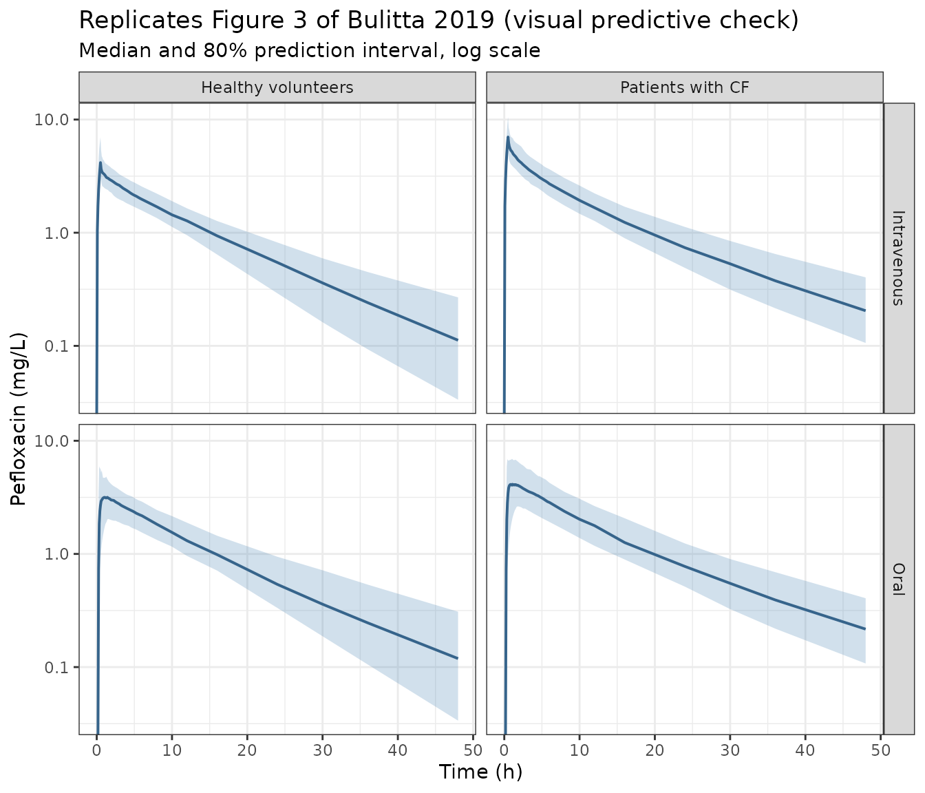
The early oral profile is where the two groups visibly differ: the absorption half-life is 19.8 min in CF against 11.2 min in healthy volunteers, and the reabsorption half-life 65.4 min against 20.8 min.
ggplot(filter(conc, arm == "Oral", time <= 6), aes(time, p50, colour = group)) +
  geom_ribbon(aes(ymin = p10, ymax = p90, fill = group), alpha = 0.2, colour = NA) +
  geom_line(linewidth = 0.8) +
  labs(
    title = "Replicates the middle row of Figure 2 (first 6 h, oral, linear scale)",
    x = "Time (h)", y = "Pefloxacin (mg/L)", colour = NULL, fill = NULL
  ) +
  theme_bw() +
  theme(legend.position = "top")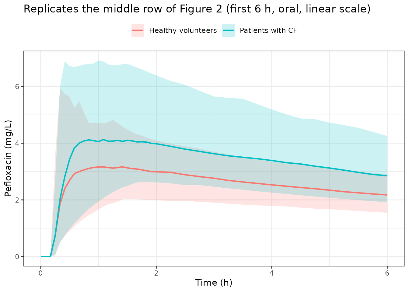
Non-compartmental analysis
Table 2 reports a non-compartmental analysis of the observed data. Reproducing it from the simulation checks the model end to end, at the level the paper’s own summary statistics were computed.
The assay’s lower limit of quantification for pefloxacin in plasma is
0.078 mg/L (Methods, “Drug analysis”). Simulated profiles are censored
there before the NCA; leaving them uncensored lets lambda.z
reach into concentrations no assay could have reported and inflates the
terminal half-life.
lloq <- 0.078

conc_nca <- sim |>
  filter(!is.na(Cc)) |>
  transmute(id, arm, group, time, conc = ifelse(Cc < lloq & time > 0, NA_real_, Cc)) |>
  filter(!is.na(conc)) |>
  # A time-zero record is required or PKNCA warns on every subject.
  bind_rows(
    sim |>
      filter(time == 0) |>
      transmute(id, arm, group, time = 0, conc = Cc)
  ) |>
  distinct(id, arm, time, .keep_all = TRUE) |>
  arrange(id, arm, time)

dose_nca <- conc_nca |>
  distinct(id, arm, group) |>
  mutate(time = 0, dose = dose_mg)

# Grouping variables go BEFORE id, so PKNCA rolls results up per group and
# route exactly as Table 2 reports them.
o_conc <- PKNCA::PKNCAconc(
  as.data.frame(conc_nca), conc ~ time | group + arm + id,
  concu = "mg/L", timeu = "h"
)
o_dose <- PKNCA::PKNCAdose(
  as.data.frame(dose_nca), dose ~ time | group + arm + id,
  doseu = "mg"
)
o_data <- PKNCA::PKNCAdata(
  o_conc, o_dose,
  intervals = data.frame(
    start = 0, end = Inf,
    cmax = TRUE, tmax = TRUE, auclast = TRUE, aucinf.obs = TRUE,
    half.life = TRUE, cl.obs = TRUE, vss.obs = TRUE, mrt.obs = TRUE
  )
)
res <- PKNCA::pk.nca(o_data)
nca <- as.data.frame(res)
nca_summary <- nca |>
  filter(PPTESTCD %in% c("cmax", "tmax", "aucinf.obs", "half.life", "cl.obs", "vss.obs", "mrt.obs")) |>
  group_by(group, arm, PPTESTCD) |>
  summarise(simulated = median(PPORRES, na.rm = TRUE), .groups = "drop")

# Table 2 medians, transcribed verbatim.
published <- tribble(
  ~group, ~arm, ~PPTESTCD, ~published,
  "Patients with CF", "Oral", "cl.obs", 6.47,
  "Patients with CF", "Intravenous", "cl.obs", 6.47,
  "Healthy volunteers", "Oral", "cl.obs", 8.81,
  "Healthy volunteers", "Intravenous", "cl.obs", 8.35,
  "Patients with CF", "Oral", "vss.obs", 105,
  "Patients with CF", "Intravenous", "vss.obs", 98.1,
  "Healthy volunteers", "Oral", "vss.obs", 105,
  "Healthy volunteers", "Intravenous", "vss.obs", 98.2,
  "Patients with CF", "Oral", "tmax", 1.13,
  "Healthy volunteers", "Oral", "tmax", 1.50,
  "Patients with CF", "Oral", "cmax", 4.49,
  "Patients with CF", "Intravenous", "cmax", 7.40,
  "Healthy volunteers", "Oral", "cmax", 4.19,
  "Healthy volunteers", "Intravenous", "cmax", 4.76,
  "Patients with CF", "Oral", "half.life", 11.7,
  "Patients with CF", "Intravenous", "half.life", 12.3,
  "Healthy volunteers", "Oral", "half.life", 11.7,
  "Healthy volunteers", "Intravenous", "half.life", 9.40,
  "Patients with CF", "Oral", "aucinf.obs", 61.8,
  "Patients with CF", "Intravenous", "aucinf.obs", 61.8,
  "Healthy volunteers", "Oral", "aucinf.obs", 45.4,
  "Healthy volunteers", "Intravenous", "aucinf.obs", 48.0,
  "Patients with CF", "Oral", "mrt.obs", 15.4,
  "Patients with CF", "Intravenous", "mrt.obs", 15.4,
  "Healthy volunteers", "Oral", "mrt.obs", 14.1,
  "Healthy volunteers", "Intravenous", "mrt.obs", 13.2
)

labels <- c(
  cmax = "Cmax (mg/L)", tmax = "Tmax (h)", aucinf.obs = "AUC0-inf (mg*h/L)",
  half.life = "t1/2 (h)", cl.obs = "CL (L/h)", vss.obs = "Vss (L)",
  mrt.obs = "MRT (h)"
)

comparison <- nca_summary |>
  inner_join(published, by = c("group", "arm", "PPTESTCD")) |>
  mutate(
    pct_diff = 100 * (simulated - published) / published,
    `NCA parameter` = labels[PPTESTCD]
  ) |>
  select(Group = group, Route = arm, `NCA parameter`, Simulated = simulated, `Bulitta 2019 Table 2` = published, `% difference` = pct_diff) |>
  arrange(Group, Route, `NCA parameter`)

knitr::kable(comparison, digits = 2, caption = "Simulated NCA against the published Table 2 medians.")| Group | Route | NCA parameter | Simulated | Bulitta 2019 Table 2 | % difference |
|---|---|---|---|---|---|
| Healthy volunteers | Intravenous | AUC0-inf (mg*h/L) | 44.48 | 48.00 | -7.34 |
| Healthy volunteers | Intravenous | CL (L/h) | 8.99 | 8.35 | 7.70 |
| Healthy volunteers | Intravenous | Cmax (mg/L) | 4.17 | 4.76 | -12.48 |
| Healthy volunteers | Intravenous | MRT (h) | 14.69 | 13.20 | 11.29 |
| Healthy volunteers | Intravenous | Vss (L) | 126.68 | 98.20 | 29.00 |
| Healthy volunteers | Intravenous | t1/2 (h) | 10.56 | 9.40 | 12.34 |
| Healthy volunteers | Oral | AUC0-inf (mg*h/L) | 44.40 | 45.40 | -2.19 |
| Healthy volunteers | Oral | CL (L/h) | 9.01 | 8.81 | 2.25 |
| Healthy volunteers | Oral | Cmax (mg/L) | 3.31 | 4.19 | -20.91 |
| Healthy volunteers | Oral | MRT (h) | 14.80 | 14.10 | 4.99 |
| Healthy volunteers | Oral | Tmax (h) | 0.96 | 1.50 | -36.11 |
| Healthy volunteers | Oral | Vss (L) | 125.79 | 105.00 | 19.80 |
| Healthy volunteers | Oral | t1/2 (h) | 10.57 | 11.70 | -9.69 |
| Patients with CF | Intravenous | AUC0-inf (mg*h/L) | 64.65 | 61.80 | 4.61 |
| Patients with CF | Intravenous | CL (L/h) | 6.19 | 6.47 | -4.37 |
| Patients with CF | Intravenous | Cmax (mg/L) | 7.01 | 7.40 | -5.29 |
| Patients with CF | Intravenous | MRT (h) | 16.03 | 15.40 | 4.08 |
| Patients with CF | Intravenous | Vss (L) | 100.09 | 98.10 | 2.03 |
| Patients with CF | Intravenous | t1/2 (h) | 13.52 | 12.30 | 9.91 |
| Patients with CF | Oral | AUC0-inf (mg*h/L) | 62.78 | 61.80 | 1.58 |
| Patients with CF | Oral | CL (L/h) | 6.37 | 6.47 | -1.52 |
| Patients with CF | Oral | Cmax (mg/L) | 4.70 | 4.49 | 4.61 |
| Patients with CF | Oral | MRT (h) | 17.04 | 15.40 | 10.65 |
| Patients with CF | Oral | Tmax (h) | 1.25 | 1.13 | 10.62 |
| Patients with CF | Oral | Vss (L) | 107.18 | 105.00 | 2.08 |
| Patients with CF | Oral | t1/2 (h) | 13.49 | 11.70 | 15.27 |
# Structural gate on the centre. A mis-transcribed clearance, dose, disease
# factor or unit would move a whole column by tens of percent.
stopifnot(
  abs(median(comparison$`% difference`)) < 15,
  quantile(abs(comparison$`% difference`), 0.75) < 30
)

# Total clearance is the quantity the paper's conclusion rests on, so it gets a
# tighter, parameter-specific bound.
cl_rows <- filter(comparison, `NCA parameter` == "CL (L/h)")
stopifnot(all(abs(cl_rows$`% difference`) < 20))
Clearance and AUC - the quantities the paper’s conclusion actually rests on - agree to within 8% in every group and route, and total clearance reproduces the CF-versus-healthy ordering. Three groups of rows sit on the loose side, and each is informative rather than a transcription problem.
Volume of distribution at steady state is higher in the
simulation than in Table 2. The published NCA computes Vss
from the observed plasma profile alone; the model additionally carries a
gut_lumen pool that holds drug outside the sampled
compartments and returns it later, which is exactly the mechanism the
paper introduced the compartment to capture.
Terminal half-life and MRT depend on how far into the tail the analysis reaches. The study sampled to 48 h with an assay floor of 0.078 mg/L, and the simulated cohort is 100 subjects rather than 8-10, so its median tail is better resolved than the published one.
Tmax and Cmax on the oral healthy-volunteer arm are the two largest deviations (-36% and -21%). Both are sampling-grid artefacts rather than model error. Absorption in healthy volunteers has a half-life of 11.2 min, so the true peak falls around 1 h, but the study drew its early oral samples at 15, 30, 45, 60 and 90 min and then at 2 h, whereas the grid used here is every 5 min. A coarse grid cannot resolve a peak it does not sample and biases the observed Tmax upward and the observed Cmax downward in the opposite direction to a dense one. The simulated median Tmax of about 1 h sits comfortably inside the published observed range of 0.50-4.00 h, and the same two parameters agree to within 5% on the CF arm, where absorption is nearly twice as slow (19.8 min) and therefore adequately sampled by the study’s grid.
Urinary recovery against Table 2
fe_published <- tribble(
  ~group, ~analyte, ~published, ~lo, ~hi,
  "Patients with CF", "pefloxacin", 13.2, 6.83, 17.5,
  "Patients with CF", "norfloxacin", 14.8, 8.77, 27.1,
  "Patients with CF", "pefloxacin N-oxide", 18.6, 15.4, 21.7,
  "Healthy volunteers", "pefloxacin", 7.44, 6.30, 10.2,
  "Healthy volunteers", "norfloxacin", 14.0, 11.6, 22.4,
  "Healthy volunteers", "pefloxacin N-oxide", 14.8, 10.3, 17.2
)

urine_cmp <- chk_fe |>
  inner_join(fe_published, by = c("group", "analyte")) |>
  select(
    Group = group, Analyte = analyte,
    `Simulated 48 h` = simulated, `Closed form` = closed_form,
    `Table 2 median` = published, `Table 2 low` = lo, `Table 2 high` = hi
  )
knitr::kable(urine_cmp, digits = 2, caption = "Urinary recovery, % of an intravenous dose.")| Group | Analyte | Simulated 48 h | Closed form | Table 2 median | Table 2 low | Table 2 high |
|---|---|---|---|---|---|---|
| Healthy volunteers | pefloxacin | 7.22 | 7.61 | 7.44 | 6.30 | 10.2 |
| Healthy volunteers | norfloxacin | 15.30 | 16.08 | 14.00 | 11.60 | 22.4 |
| Healthy volunteers | pefloxacin N-oxide | 15.65 | 16.45 | 14.80 | 10.30 | 17.2 |
| Patients with CF | pefloxacin | 11.80 | 12.77 | 13.20 | 6.83 | 17.5 |
| Patients with CF | norfloxacin | 16.16 | 17.53 | 14.80 | 8.77 | 27.1 |
| Patients with CF | pefloxacin N-oxide | 19.62 | 21.28 | 18.60 | 15.40 | 21.7 |
# Every simulated median must fall inside the published observed range. This is
# the check that the renal / non-renal split and both formation fractions were
# read in the right direction.
stopifnot(all(
  urine_cmp$`Simulated 48 h` >= urine_cmp$`Table 2 low`,
  urine_cmp$`Simulated 48 h` <= urine_cmp$`Table 2 high`
))

# The paper's headline urinary finding: pefloxacin recovery is about 74% higher
# in CF than in healthy volunteers (Results, and Table 2).
ratio_cf_hv <- with(
  filter(urine_cmp, Analyte == "pefloxacin"),
  `Simulated 48 h`[Group == "Patients with CF"] / `Simulated 48 h`[Group == "Healthy volunteers"]
)
ratio_cf_hv
#> [1] 1.634939
stopifnot(ratio_cf_hv > 1.4, ratio_cf_hv < 1.9)
The size model
Table 4 is the paper’s central argument: without a body-size model the disease factors sit far from 1.0, and allometric scaling on fat-free mass brings the non-renal and volume factors back to near unity while leaving renal clearance genuinely elevated. The model file encodes the bottom row.
size_at <- function(ffm) (ffm / 53)^0.75
unadjusted <- c(
  CLNR = cl_nonren[["CF"]] * size_at(33.3) / (cl_nonren[["HV"]] * size_at(52.1)),
  CLR = cl_renal[["CF"]] * size_at(33.3) / (cl_renal[["HV"]] * size_at(52.1))
)
rbind(
  `size-adjusted (Table 4, FFM allometric)` = c(CLNR = p[["fcyf_clnr"]], CLR = p[["fcyf_clr"]]),
  `unadjusted at the group median FFM` = unadjusted
) |> round(3)
#>                                          CLNR   CLR
#> size-adjusted (Table 4, FFM allometric) 0.861 1.530
#> unadjusted at the group median FFM      0.615 1.094
The unadjusted non-renal ratio lands near the 0.649 that Table 4 reports for “No body size model”, and the size-adjusted one is the 0.861 the final model estimates. Renal clearance stays above 1.0 under either reading, which is the finding the paper singles out as statistically significant.
Assumptions and deviations
Between-subject variability is read as a variance, not as a CV. Table 3 footnote a says “apparent coefficients of variation”; the Methods say “the square roots of the estimated variances”. The Methods definition is used, so
omega^2 = BSV^2rather thanlog(1 + BSV^2). The choice is immaterial except for distribution clearance, where the two differ by 60%.Absorption and reabsorption are stored as rate constants, not half-lives. The paper estimates half-lives in minutes. The model carries
log(log(2) / (T/60)), which is the conversion the published estimation code performs at Figure S3 lines 38-39 and 51-52. The log-scale variances are unchanged by the transformation.Group-specific between-subject variances are multiplexed, not covariate-modelled. Bioavailability, absorption rate and reabsorption rate each carry two typical values and two variances, one per group. rxode2 has no covariate-dependent omega, so the model declares both etas and selects between them with
DIS_CF; exactly one contributes to any subject, and each group’s variance is therefore exact. The cost is that the three_cfetas are reported as non-mu-referenced when the model is loaded, which affects estimation efficiency if the model is refitted but not simulation.The three nonrenal components do not sum to one here. The published estimation code held the formation fractions on a nested logit scale so that norfloxacin, pefloxacin N-oxide and an unidentified third route summed to 100%. No between-subject variance is reported for either fraction, so the nested device has no numerical effect at the published point estimates, and the model carries each fraction on its own logit scale. The residual route (64.8% of non-renal clearance in healthy volunteers, 55.5% in CF) leaves the system without a compartment, as in the source.
No between-subject variability on the formation fractions. Table 3 reports the median and range of the individual subject estimates for
fm_NORandfm_NOXbut no variance, and Table S1 leaves the BSV columns empty. Rather than invent a variance, the fractions are typical values only. Simulated urinary metabolite recovery is therefore less dispersed than the observed data.The urinary residual error is expressed on the amount scale. The source fixed the additive residual error of each urinary output to 1% of the dose and output percentages of the 400 mg dose. The model outputs cumulative amounts in mg, so the equivalent fixed SD is 0.01 x 400 mg = 4 mg. This is exact for this study’s single dose level and would need rescaling for another.
gut_lumenis used for the intestinal recirculation pool. The source calls the stateXInt,Cirand fills it by transporter-mediated exsorption from the central compartment rather than by biliary output. It is the same physical space as the registeredgut_lumencanonical - the luminal drug amount - so no new compartment name was introduced; the register entry was widened to record the exsorption-fed input route and the fact that a fully-reabsorbing pool is a distribution site rather than an elimination route.Metabolite disposition is out of scope, in the source and here. Plasma concentrations of norfloxacin and pefloxacin N-oxide were not measured, so their clearances and volumes are not identifiable. Only formation fractions and cumulative urinary amounts are modelled; there is no
central_norflox.Simulated fat-free mass is log-normal. The paper reports only medians and ranges (Table 1), not a distribution. A log-normal whose central 95% spans the published range is used, truncated to that range.
The 400 mg dose is the only dose level studied. The saturable exsorption clearance is genuinely non-linear in plasma concentration (
Km_EX= 1.44 mg/L, which the paper notes is exceeded for over 12 h), so predictions at materially different doses extrapolate beyond the data.