Meropenem (Kim 2024) • nlmixr2lib

Model and source

Citation: Kim YK, Kang G, Zang DY, Lee DH. (2024). Precision Dosing of Meropenem in Adults with Normal Renal Function: Insights from a Population Pharmacokinetic and Monte Carlo Simulation Study. Antibiotics 13(9):849. doi:10.3390/antibiotics13090849.
Description: Two-compartment intravenous population PK model for meropenem in healthy Korean adults with normal renal function (Kim 2024; n = 12, 84 plasma samples after a single 500 mg 30-min IV infusion). Total clearance depends on serum creatinine through a power model centred at the cohort median 0.86 mg/dL: CL = 12.4 * (CREAT/0.86)^-0.392 L/h, so CL falls from 14.3 L/h at CREAT = 0.6 mg/dL to 11.7 L/h at CREAT = 1.0 mg/dL. Because the estimated correlation between the random effects on CL and Vc was 0.99, the paper codes a SINGLE eta shared by both parameters, with the Vc random effect constructed as 1.53 * eta_CL (Table 2 ‘V1’ row under interindividual variability). Interindividual variability on Q and Vp is fixed, not estimated. Residual error is proportional. The unbound concentration Cu = fu * Cc (fu = 0.98) is the driver of the fT>MIC PK/PD targets (40% fT>MIC, 40% fT>4MIC, 100% fT>MIC, 100% fT>4MIC) used in the paper’s Monte Carlo probability-of-target-attainment simulations for intermittent, 3-h extended, and continuous infusion regimens.
Article: Antibiotics 2024;13(9):849
Supplement (Figures S1-S2, Tables S1-S2): https://www.mdpi.com/article/10.3390/antibiotics13090849/s1

Meropenem is a carbapenem beta-lactam whose efficacy is driven by the time the free drug concentration stays above the MIC (%fT>MIC). Most published meropenem population PK models come from critically ill patients with impaired or supported renal function; Kim and colleagues instead fitted healthy Korean adults with normal renal function, then used the model in Monte Carlo simulations to ask whether the standard 1 g every 8 h regimen is adequate when renal function is normal.

Population

Fourteen healthy volunteers consented and 12 were analysed (two were excluded after positive allergic skin tests). The cohort was 4 female and 8 male, mean age 36.8 years (CV 19.9%; protocol range 19-55), mean weight 65.7 kg (CV 20.8%), mean body surface area 1.74 m^2 (Table 1). Renal function was normal by every measure reported: Cockcroft-Gault creatinine clearance 105 mL/min (CV 21.2%), BSA-normalized 93.8 mL/min/1.73 m^2, CKD-EPI creatinine eGFR 111 mL/min/1.73 m^2. Serum creatinine averaged 0.863 mg/dL (CV 19.0%; median 0.860, IQR 0.738-1.02), and that median is the centring value of the covariate model.

Each participant received a single 500 mg dose of meropenem in 100 mL of saline infused intravenously over 30 minutes, with plasma sampled pre-dose and at 0.5, 0.75, 1, 2, 3 and 6 h from the start of the infusion (84 samples in total). Estimation used NONMEM 7.5 with FOCE-I and subroutine ADVAN3 TRANS4; PsN 5.3.1 provided the stepwise covariate search, the VPC and a 2000-sample nonparametric bootstrap.

The same information is available programmatically via the model’s population metadata (readModelDb("Kim_2024_meropenem")()$population).

Source trace

The per-parameter origin is recorded as an in-file comment next to each ini() entry in inst/modeldb/specificDrugs/Kim_2024_meropenem.R. The table below collects them in one place for review.

Equation / parameter	Value as published	Value in `ini()`	Source location
`lcl`	theta1 = 12.4 L/h (RSE 7.87%; bootstrap 12.3, 95% CI 10.8-14.7)	`log(12.4)`	Table 2, structural model
`lvc`	V1 = 8.26 L (RSE 12.5%; bootstrap 8.31, 95% CI 6.56-11.0)	`log(8.26)`	Table 2
`lq`	Q = 5.22 L/h (RSE 16.1%; bootstrap 5.05, 95% CI 3.34-7.33)	`log(5.22)`	Table 2
`lvp`	V2 = 4.06 L (RSE 11.1%; bootstrap 4.01, 95% CI 3.00-5.07)	`log(4.06)`	Table 2
`e_creat_cl`	theta2 = -0.392 (RSE 19.2%; bootstrap -0.378, 95% CI -0.579 to -0.115)	`-0.392`	Table 2, structural model
CL covariate form	`CL = theta1 * (CR/0.86)^theta2`	`exp(lcl + etalcl) * (CREAT/0.86)^e_creat_cl`	Table 2, structural-model row
Reference creatinine	0.86 mg/dL (cohort median 0.860)	`0.86` in `model()`	Table 2 equation; Table 1
`etalcl`	IIV on CL = 26.2% (RSE 30.4%, shrinkage 1.82%)	`0.0663906` = `log(1 + 0.262^2)`	Table 2
`scale_etalvc`	V1 row = 1.53 (RSE 4.80%; bootstrap 1.53, 95% CI 1.07-2.43)	`1.53`	Table 2 IIV block + footnote a; Results 2.2
`etalq`	IIV on Q = 14.4%, fixed (shrinkage 49.1%)	`fixed(0.0205239)` = `log(1 + 0.144^2)`	Table 2, footnote b
`etalvp`	IIV on V2 = 17.9%, fixed (shrinkage 11.2%)	`fixed(0.0315384)` = `log(1 + 0.179^2)`	Table 2, footnote b
`propSd`	proportional error 10.9% (RSE 20.4%; bootstrap 10.4, 95% CI 6.50-14.0)	`0.109`	Table 2
`fu`	“The fraction of unbound drug (f) was fixed at 0.98”	`fixed(0.98)`	Methods 4.5, Dosage Simulation
`d/dt(central)`, `d/dt(peripheral1)`	two-compartment model, ADVAN3 TRANS4	n/a	Results 2.2; Methods 4.3
`Cu <- fu * Cc`	%fT>MIC computed on free drug	n/a	Methods 4.5; Results 2.4

Results 2.2 explains the shared random effect: the correlation between the CL and V1 variabilities was 0.99, so the authors coded a single eta, with CL = TVCL * EXP[ETA(1)] and V1 = TVV1 * EXP[THETA(1) * ETA(1)], and estimated THETA(1) at 1.53 in the final model. That is scale_etalvc here; there is no independent eta on vc.

Virtual cohort

Original participant-level data are not public. The simulations below use a virtual cohort of 200 adults whose serum creatinine matches the Table 1 distribution (mean 0.863 mg/dL, CV 19.0%), drawn from a lognormal distribution as the paper’s own Monte Carlo simulations did (“assuming a lognormal distribution for each parameter or covariate”, Methods 4.5).

set.seed(20240905)

n_sub    <- 200L
creat_mn <- 0.863
creat_cv <- 0.190

creat_sdlog  <- sqrt(log(1 + creat_cv^2))
creat_meanlog <- log(creat_mn) - creat_sdlog^2 / 2

pop <- tibble::tibble(
  id    = seq_len(n_sub),
  CREAT = stats::rlnorm(n_sub, creat_meanlog, creat_sdlog)
)

tibble::tibble(
  Statistic = c("Mean (mg/dL)", "CV (%)", "Median (mg/dL)", "IQR (mg/dL)"),
  Simulated = c(
    sprintf("%.3f", mean(pop$CREAT)),
    sprintf("%.1f", 100 * stats::sd(pop$CREAT) / mean(pop$CREAT)),
    sprintf("%.3f", stats::median(pop$CREAT)),
    sprintf("%.3f-%.3f", stats::quantile(pop$CREAT, 0.25), stats::quantile(pop$CREAT, 0.75))
  ),
  `Kim 2024 Table 1` = c("0.863", "19.0", "0.860", "0.738-1.02")
) |>
  knitr::kable(caption = "Virtual-cohort serum creatinine vs. the published cohort.")

Virtual-cohort serum creatinine vs. the published cohort.
Statistic	Simulated	Kim 2024 Table 1
Mean (mg/dL)	0.874	0.863
CV (%)	19.9	19.0
Median (mg/dL)	0.859	0.860
IQR (mg/dL)	0.747-0.978	0.738-1.02

Simulation

mod <- readModelDb("Kim_2024_meropenem")

# The variance-covariance matrix of the random effects, captured once so that
# every population solve below can pass it explicitly. rxode2 caches the
# solve-time `omega` against the compiled model, so a later solve inherits
# whatever the previous one used -- including the `omega = NA` of the
# typical-value chunk, which would silently strip the between-subject
# variability from the population runs.
mod_omega <- rxode2::rxode(mod)$omega
#> ℹ parameter labels from comments will be replaced by 'label()'
mod_omega
#>           etalcl     etalq    etalvp
#> etalcl 0.0663906 0.0000000 0.0000000
#> etalq  0.0000000 0.0205239 0.0000000
#> etalvp 0.0000000 0.0000000 0.0315384
#> attr(,"lotriLabels")
#> [1] "Table 2: IIV on CL = 26.2% (RSE 30.4%, shrinkage 1.82%; bootstrap 25.4%, 95% CI 7.8-38.3) -> log(1 + 0.262^2)"
#> [2] "Table 2: IIV on Q = 14.4% (footnote b: fixed; shrinkage 49.1%) -> log(1 + 0.144^2)"                           
#> [3] "Table 2: IIV on V2 = 17.9% (footnote b: fixed; shrinkage 11.2%) -> log(1 + 0.179^2)"                          
#> attr(,"lotriFix")
#>        etalcl etalq etalvp
#> etalcl  FALSE FALSE  FALSE
#> etalq   FALSE  TRUE  FALSE
#> etalvp  FALSE FALSE   TRUE

Typical-value check of the covariate model

The Discussion prints two anchor points for the creatinine relationship: CL is 14.3 L/h at a serum creatinine of 0.6 mg/dL and 11.7 L/h at 1.0 mg/dL. Both are reproduced exactly by 12.4 * (CREAT/0.86)^-0.392, and the reported steady-state volume of distribution (Vss = V1 + V2 = 12.32 L) is likewise exact.

The typical-value solve passes omega = NA rather than calling rxode2::zeroRe(): zeroRe() mutates state shared with the compiled model, so whichever kind of solve runs first in a session wins for the rest of it. omega = NA affects only this solve, so chunk order cannot silently strip the between-subject variability from the population runs below.

creat_anchor <- c(0.6, 0.86, 1.0)

typ_cl <- vapply(creat_anchor, function(cr) {
  ev <- dplyr::bind_rows(
    tibble::tibble(time = 0, amt = 500, dur = 0.5, evid = 1L, cmt = "central"),
    tibble::tibble(time = c(0, 0.5, 1), amt = NA_real_, dur = NA_real_,
                   evid = 0L, cmt = "central")
  ) |>
    dplyr::mutate(CREAT = cr) |>
    dplyr::arrange(time, dplyr::desc(evid))
  s <- rxode2::rxSolve(mod, events = ev, omega = NA) |> as.data.frame()
  stopifnot(dplyr::n_distinct(round(s$cl, 10)) == 1L)  # etas really are zero
  s$cl[1]
}, numeric(1))
#> ℹ parameter labels from comments will be replaced by 'label()'

typ_vc <- {
  ev <- dplyr::bind_rows(
    tibble::tibble(time = 0, amt = 500, dur = 0.5, evid = 1L, cmt = "central"),
    tibble::tibble(time = 1, amt = NA_real_, dur = NA_real_, evid = 0L, cmt = "central")
  ) |>
    dplyr::mutate(CREAT = 0.86)
  s <- rxode2::rxSolve(mod, events = ev, omega = NA) |> as.data.frame()
  c(vc = s$vc[1], vp = s$vp[1], q = s$q[1])
}

tibble::tibble(
  Quantity = c("CL at CREAT = 0.6 mg/dL (L/h)",
               "CL at CREAT = 0.86 mg/dL (L/h)",
               "CL at CREAT = 1.0 mg/dL (L/h)",
               "Vss = V1 + V2 (L)"),
  Simulated = sprintf("%.2f", c(typ_cl, typ_vc[["vc"]] + typ_vc[["vp"]])),
  Published = c("14.3 (Discussion)", "12.4 (Table 2 theta1)",
                "11.7 (Discussion)", "12.32 (Discussion)")
) |>
  knitr::kable(caption = "Typical-value reproduction of the published covariate relationship.")

Typical-value reproduction of the published covariate relationship.
Quantity	Simulated	Published
CL at CREAT = 0.6 mg/dL (L/h)	14.28	14.3 (Discussion)
CL at CREAT = 0.86 mg/dL (L/h)	12.40	12.4 (Table 2 theta1)
CL at CREAT = 1.0 mg/dL (L/h)	11.69	11.7 (Discussion)
Vss = V1 + V2 (L)	12.32	12.32 (Discussion)


stopifnot(
  abs(typ_cl[1] - 14.3) < 0.05,
  abs(typ_cl[2] - 12.4) < 1e-8,
  abs(typ_cl[3] - 11.7) < 0.05,
  abs(typ_vc[["vc"]] + typ_vc[["vp"]] - 12.32) < 1e-8
)

Single 500 mg 30-min infusion (the estimation study)

# The paper's own sampling schedule (Methods 4.2), plus a denser grid used only
# for the figure.
nca_times  <- c(0, 0.5, 0.75, 1, 2, 3, 6)
plot_times <- sort(unique(c(nca_times, seq(0, 0.5, by = 0.05), seq(0.6, 6, by = 0.1))))

make_single <- function(times) {
  dplyr::bind_rows(
    pop |> dplyr::mutate(time = 0, amt = 500, dur = 0.5, evid = 1L, cmt = "central"),
    pop |> tidyr::crossing(tibble::tibble(time = times)) |>
      dplyr::mutate(amt = NA_real_, dur = NA_real_, evid = 0L, cmt = "central")
  ) |>
    dplyr::arrange(id, time, dplyr::desc(evid))
}

solve_pop <- function(ev, label) {
  s <- rxode2::rxSolve(mod, events = ev, keep = c("CREAT"), omega = mod_omega) |>
    as.data.frame()
  # Guards (see the rxSolve caveats in the nlmixr2lib skill notes): every
  # subject must come back, every concentration must be finite, and the
  # between-subject variability must actually be present.
  if (dplyr::n_distinct(s$id) != n_sub) {
    stop("rxSolve dropped subjects in arm: ", label)
  }
  if (!all(is.finite(s$Cc))) stop("non-finite concentrations in arm: ", label)
  per_sub <- unique(data.frame(id = s$id, cl = s$cl, CREAT = s$CREAT))
  # cl = exp(lcl + eta) * (CREAT/0.86)^theta2, so removing the covariate term
  # leaves exp(lcl + eta); its log-SD must be the published 0.2577.
  if (stats::sd(log(per_sub$cl) + 0.392 * log(per_sub$CREAT / 0.86)) < 0.1) {
    stop("between-subject variability was dropped in arm: ", label)
  }
  s
}

sim_plot <- solve_pop(make_single(plot_times), "single 500 mg")
sim_nca_raw <- solve_pop(make_single(nca_times), "single 500 mg (NCA grid)")

Concentration-time profile (Figure S2 / Figure 1 analogue)

Kim 2024 shows the observed-vs-predicted diagnostics in Figure 1 and the visual predictive check in Figure S2; neither tabulates the underlying concentrations, so only the model side can be reproduced. The overlay below is the published Table 3 NCA summary: Cmax 40.2 mg/L at the end of the 30-min infusion, and Clast 0.393 mg/L at a mean Tlast of 5.83 h.

obs_points <- tibble::tibble(
  time = c(0.5, 5.83),
  Cc   = c(40.2, 0.393),
  what = "Table 3 mean (Cmax; Clast at mean Tlast)"
)

sim_plot |>
  dplyr::filter(time > 0) |>
  dplyr::group_by(time) |>
  dplyr::summarise(
    Q05 = stats::quantile(Cc, 0.05),
    Q50 = stats::quantile(Cc, 0.50),
    Q95 = stats::quantile(Cc, 0.95),
    .groups = "drop"
  ) |>
  ggplot2::ggplot(ggplot2::aes(time, Q50)) +
  ggplot2::geom_ribbon(ggplot2::aes(ymin = Q05, ymax = Q95), alpha = 0.2) +
  ggplot2::geom_line(linewidth = 0.9) +
  ggplot2::geom_point(data = obs_points, ggplot2::aes(time, Cc, shape = what),
                      size = 3, inherit.aes = FALSE) +
  ggplot2::scale_y_log10() +
  ggplot2::scale_shape_manual(values = 4) +
  ggplot2::labs(
    x = "Time (h)", y = "Meropenem concentration (mg/L)",
    shape = NULL,
    title = "Simulated single 500 mg 30-min IV infusion (median and 5th-95th percentile)",
    caption = "Model side of Kim 2024 Figure S2; markers are the Table 3 NCA summary."
  ) +
  ggplot2::theme(legend.position = "bottom")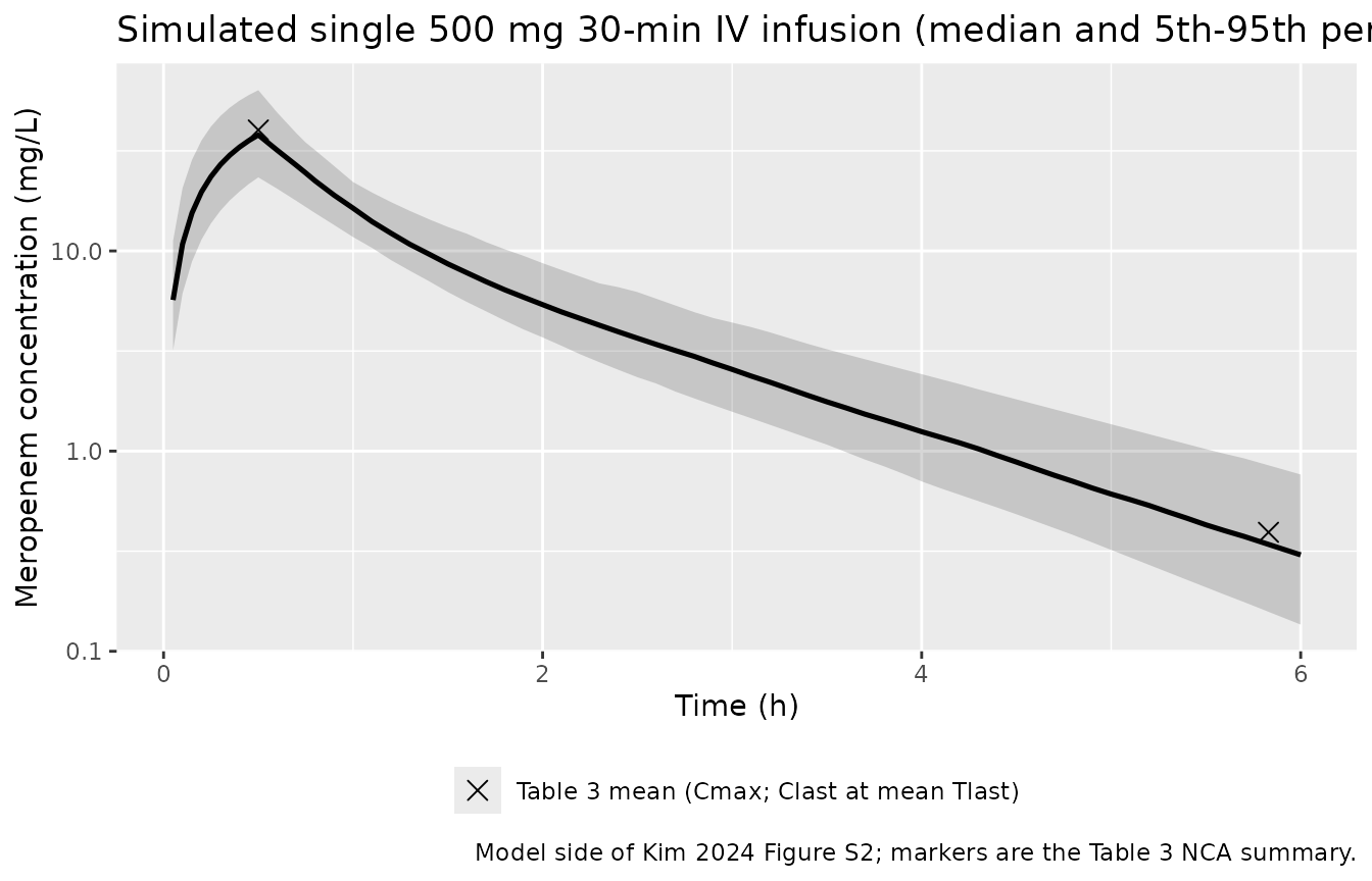

PKNCA validation

The NCA is run on the paper’s own sampling schedule so that the extrapolation behaviour matches: AUC by linear-up / log-down trapezoid, aucinf.obs extrapolated from the last observed concentration, and half-life from the log-linear terminal phase.

sim_nca <- sim_nca_raw |>
  dplyr::filter(!is.na(Cc)) |>
  dplyr::mutate(treatment = "500 mg, 30-min IV infusion") |>
  dplyr::select(id, time, Cc, treatment)

# Guarantee a time-zero record per subject (an IV pre-dose concentration is 0).
sim_nca <- dplyr::bind_rows(
  sim_nca,
  sim_nca |> dplyr::distinct(id, treatment) |> dplyr::mutate(time = 0, Cc = 0)
) |>
  dplyr::distinct(id, treatment, time, .keep_all = TRUE) |>
  dplyr::arrange(id, treatment, time)

conc_obj <- PKNCA::PKNCAconc(sim_nca, Cc ~ time | treatment + id,
                             concu = "mg/L", timeu = "h")

dose_df <- pop |>
  dplyr::mutate(time = 0, amt = 500, dur = 0.5,
                treatment = "500 mg, 30-min IV infusion") |>
  dplyr::select(id, time, amt, dur, treatment)

# `duration` is required for the IV-infusion parameters: mrt.iv.obs subtracts
# half the infusion duration and vss.iv.obs inherits that correction.
dose_obj <- PKNCA::PKNCAdose(dose_df, amt ~ time | treatment + id, doseu = "mg",
                             route = "intravascular", duration = "dur")

intervals <- data.frame(
  start = 0, end = Inf,
  cmax = TRUE, tmax = TRUE, auclast = TRUE, aucinf.obs = TRUE,
  half.life = TRUE, mrt.iv.obs = TRUE, cl.obs = TRUE, vss.iv.obs = TRUE
)

nca_res <- PKNCA::pk.nca(PKNCA::PKNCAdata(conc_obj, dose_obj, intervals = intervals))

Comparison against published NCA

Kim 2024 Table 3 reports the NCA means over the 12 participants. CL_NCA and Vss_NCA are printed per kilogram of body weight (0.201 L/h/kg and 0.219 L/kg); the Discussion converts them to a 70 kg subject as 14.07 L/h and 15.44 L, and those are the values used as the reference here. Note that the final model has no body-weight covariate (weight was screened and not retained), so the simulated cohort carries no weight variation and the CL / Vss rows compare a weight-free model against a weight-normalized observation – see the Assumptions section.

published <- tibble::tribble(
  ~treatment,                    ~cmax, ~tmax, ~auclast, ~aucinf.obs, ~half.life, ~mrt.iv.obs, ~cl.obs, ~vss.iv.obs,
  "500 mg, 30-min IV infusion",   40.2,   0.5,     39.8,        40.4,      0.967,        1.09,   14.07,       15.44
)

cmp <- nlmixr2lib::ncaComparisonTable(
  simulated = nca_res,
  reference = published,
  by        = "treatment",
  units     = c(cmax = "mg/L", tmax = "h", auclast = "mg*h/L",
                aucinf.obs = "mg*h/L", half.life = "h", mrt.iv.obs = "h",
                cl.obs = "L/h", vss.iv.obs = "L"),
  tolerance_pct = 20
)

knitr::kable(
  cmp,
  caption = paste(
    "Simulated vs. Kim 2024 Table 3 (NCA means; CL and Vss on the 70 kg basis",
    "given in the Discussion). * differs from reference by >20%."
  ),
  align = c("l", "l", "r", "r", "r")
)

Simulated vs. Kim 2024 Table 3 (NCA means; CL and Vss on the 70 kg basis given in the Discussion). * differs from reference by >20%.
NCA parameter	treatment	Reference	Simulated	% diff
Cmax (mg/L)	500 mg, 30-min IV infusion	40.2	37.1	-7.8%
Tmax (h)	500 mg, 30-min IV infusion	0.5	0.5	+0.0%
AUC0-∞ (obs) (mg*h/L)	500 mg, 30-min IV infusion	40.4	38.6	-4.4%
AUClast (mg*h/L)	500 mg, 30-min IV infusion	39.8	38.1	-4.3%
t½ (h)	500 mg, 30-min IV infusion	0.967	0.969	+0.2%
CL/F (L/h)	500 mg, 30-min IV infusion	14.1	12.9	-8.0%
MRT (IV) (h)	500 mg, 30-min IV infusion	1.09	1.1	+0.8%
Vss (IV) (L)	500 mg, 30-min IV infusion	15.4	13.9	-9.8%

A closed-form cross-check that does not depend on the simulation at all: for a linear model with intravenous input, AUCinf = Dose / CL. At the reference creatinine, 500 / 12.4 = 40.3 mg*h/L, against the published mean AUCinf of 40.4 mg*h/L – a 0.2% agreement that confirms both the clearance value and the dose / concentration unit chain.

stopifnot(abs(500 / 12.4 - 40.4) / 40.4 < 0.01)

The two-compartment disposition half-lives implied by the published parameters also reproduce the Table 3 population-PK row directly:

k10 <- 12.4 / 8.26; k12 <- 5.22 / 8.26; k21 <- 5.22 / 4.06
s <- k10 + k12 + k21
alpha <- (s + sqrt(s^2 - 4 * k10 * k21)) / 2
beta  <- (s - sqrt(s^2 - 4 * k10 * k21)) / 2

tibble::tibble(
  Quantity  = c("t1/2 alpha (h)", "t1/2 beta (h)"),
  Derived   = sprintf("%.3f", log(2) / c(alpha, beta)),
  Published = c("0.260 (Table 3, population PK)", "0.985 (Table 3, population PK)")
) |>
  knitr::kable(caption = "Disposition half-lives derived from the Table 2 parameters.")

Disposition half-lives derived from the Table 2 parameters.
Quantity	Derived	Published
t1/2 alpha (h)	0.256	0.260 (Table 3, population PK)
t1/2 beta (h)	0.972	0.985 (Table 3, population PK)


stopifnot(abs(log(2) / alpha - 0.260) < 0.01, abs(log(2) / beta - 0.985) < 0.02)

Probability of target attainment

This is the paper’s principal result. Target attainment is evaluated on the free concentration Cu = fu * Cc (fu fixed at 0.98) over a dosing interval at steady state, against four targets: 40% fT>MIC, 40% fT>4MIC, 100% fT>MIC and 100% fT>4MIC. A regimen is considered adequate when the PTA reaches 90%.

Steady state is evaluated over the interval beginning at 24 h. With a terminal half-life near 1 h that is more than 20 half-lives of dosing, so the interval is indistinguishable from the 5-day profiles the paper simulated.

mics <- c(0.06, 0.125, 0.25, 0.5, 1, 2, 4, 8, 16)
t_ss <- 24

pta_regimen <- function(dose_mg, tau, dur_h, label) {
  dose_times <- seq(0, t_ss, by = tau)
  obs_times  <- seq(t_ss, t_ss + tau, by = 0.02)
  ev <- dplyr::bind_rows(
    pop |> tidyr::crossing(tibble::tibble(time = dose_times)) |>
      dplyr::mutate(amt = dose_mg, dur = dur_h, evid = 1L, cmt = "central"),
    pop |> tidyr::crossing(tibble::tibble(time = obs_times)) |>
      dplyr::mutate(amt = NA_real_, dur = NA_real_, evid = 0L, cmt = "central")
  ) |>
    dplyr::arrange(id, time, dplyr::desc(evid))

  s <- solve_pop(ev, label)
  obs <- s[s$evid == 0 | is.na(s$evid), , drop = FALSE]
  if (nrow(obs) == 0) obs <- s

  tidyr::expand_grid(MIC = mics,
                     target = c("40% fT>MIC", "40% fT>4MIC",
                                "100% fT>MIC", "100% fT>4MIC")) |>
    dplyr::rowwise() |>
    dplyr::mutate(
      threshold = MIC * ifelse(grepl("4MIC", target), 4, 1),
      frac_req  = ifelse(grepl("^100", target), 1, 0.40),
      PTA = 100 * mean(tapply(obs$Cu > threshold, obs$id, mean) >= frac_req - 1e-9)
    ) |>
    dplyr::ungroup() |>
    dplyr::mutate(regimen = label) |>
    dplyr::select(regimen, target, MIC, PTA)
}

Figure 2 – the current empirical regimen, 1 g every 8 h

pta_fig2 <- pta_regimen(1000, 8, 0.5, "1 g q8h, 0.5-h infusion")

pta_fig2 |>
  dplyr::mutate(target = factor(target, levels = c("40% fT>MIC", "40% fT>4MIC",
                                                   "100% fT>MIC", "100% fT>4MIC"))) |>
  ggplot2::ggplot(ggplot2::aes(MIC, PTA, colour = target, shape = target)) +
  ggplot2::geom_hline(yintercept = 90, linetype = "dashed") +
  ggplot2::geom_line() +
  ggplot2::geom_point(size = 2) +
  ggplot2::scale_x_log10(breaks = mics, labels = mics) +
  ggplot2::labs(x = "MIC (mg/L)", y = "PTA (%)", colour = NULL, shape = NULL,
                title = "1 g meropenem q8h as a 30-min infusion",
                caption = "Replicates Figure 2 of Kim 2024; dashed line is the 90% PTA criterion.") +
  ggplot2::theme(legend.position = "bottom")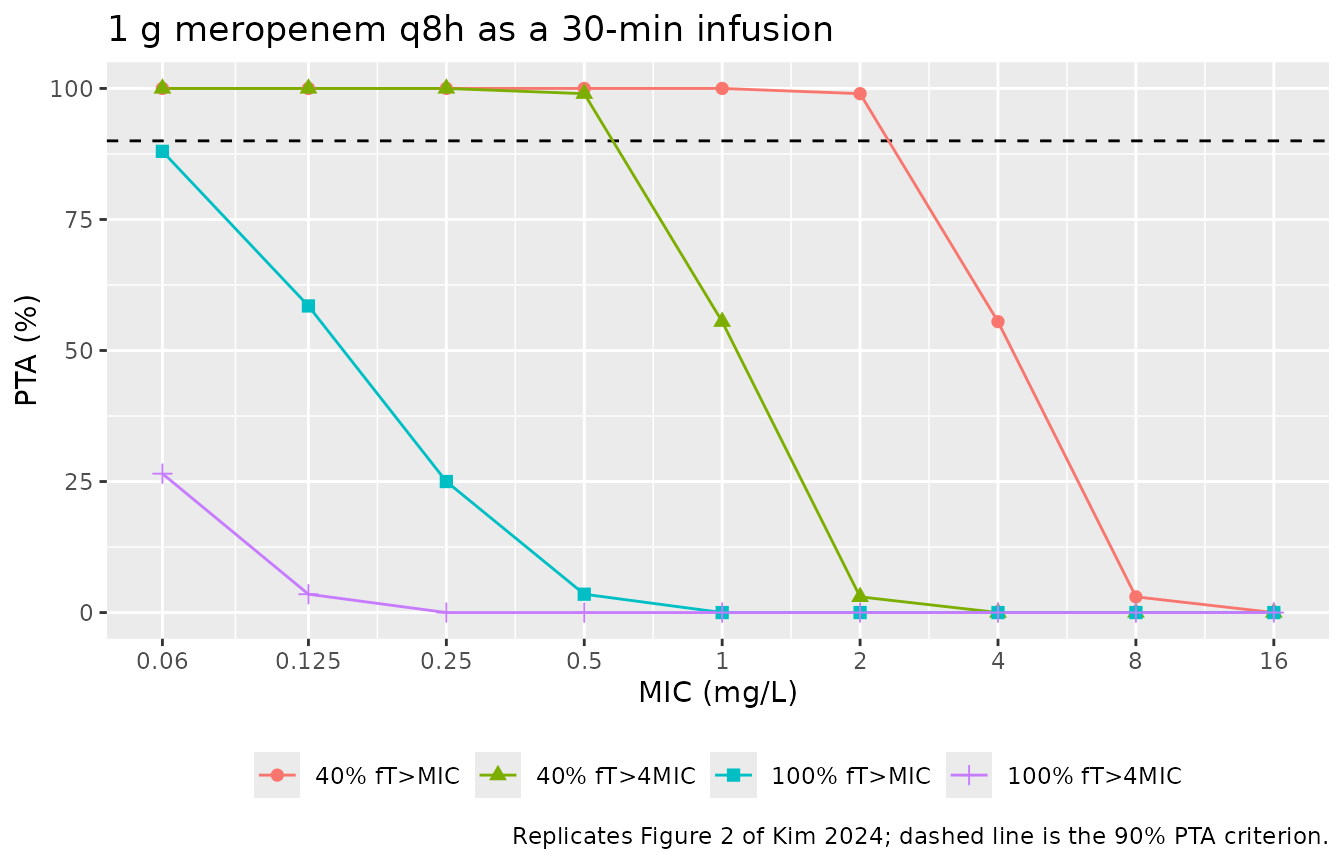

Kim 2024 makes four claims about this regimen in Results 2.4. Figure 2 is graphical only, so the claims are checked as inequalities rather than digitized values.

get_pta <- function(tbl, tgt, mic, reg = NULL) {
  x <- tbl[tbl$target == tgt & tbl$MIC == mic, ]
  if (!is.null(reg)) x <- x[x$regimen == reg, ]
  x$PTA[1]
}

claims_fig2 <- tibble::tibble(
  Claim = c(
    "90% PTA for 40% fT>MIC when MIC < 2 mg/L",
    "fails 90% PTA for 40% fT>4MIC when MIC > 1 mg/L",
    "never reaches 90% PTA for 100% fT>MIC at any MIC",
    "never reaches 90% PTA for 100% fT>4MIC at any MIC"
  ),
  `Simulated evidence` = c(
    sprintf("PTA at MIC 1 = %.1f%%; at MIC 2 = %.1f%%",
            get_pta(pta_fig2, "40% fT>MIC", 1), get_pta(pta_fig2, "40% fT>MIC", 2)),
    sprintf("PTA at MIC 1 = %.1f%%; at MIC 2 = %.1f%%",
            get_pta(pta_fig2, "40% fT>4MIC", 1), get_pta(pta_fig2, "40% fT>4MIC", 2)),
    sprintf("max PTA over all MICs = %.1f%% (at MIC %.3f)",
            max(pta_fig2$PTA[pta_fig2$target == "100% fT>MIC"]),
            pta_fig2$MIC[pta_fig2$target == "100% fT>MIC"][
              which.max(pta_fig2$PTA[pta_fig2$target == "100% fT>MIC"])]),
    sprintf("max PTA over all MICs = %.1f%%",
            max(pta_fig2$PTA[pta_fig2$target == "100% fT>4MIC"]))
  ),
  Reproduced = c(
    get_pta(pta_fig2, "40% fT>MIC", 1) >= 90,
    get_pta(pta_fig2, "40% fT>4MIC", 2) < 90,
    max(pta_fig2$PTA[pta_fig2$target == "100% fT>MIC"]) < 90,
    max(pta_fig2$PTA[pta_fig2$target == "100% fT>4MIC"]) < 90
  )
)

knitr::kable(claims_fig2, caption = "Kim 2024 Results 2.4, first simulation (Figure 2).")

Kim 2024 Results 2.4, first simulation (Figure 2).
Claim	Simulated evidence	Reproduced
90% PTA for 40% fT>MIC when MIC < 2 mg/L	PTA at MIC 1 = 100.0%; at MIC 2 = 99.0%	TRUE
fails 90% PTA for 40% fT>4MIC when MIC > 1 mg/L	PTA at MIC 1 = 55.5%; at MIC 2 = 3.0%	TRUE
never reaches 90% PTA for 100% fT>MIC at any MIC	max PTA over all MICs = 88.0% (at MIC 0.060)	TRUE
never reaches 90% PTA for 100% fT>4MIC at any MIC	max PTA over all MICs = 26.5%	TRUE

Figure 3 – intermittent and extended infusions

The paper states specific MIC ceilings for six further regimens. Each is reproduced below and compared against the published statement.

fig3_regimens <- tibble::tribble(
  ~amt,  ~ii, ~dur_h, ~label,
  1000,   12,    0.5, "1 g q12h, 0.5-h",
  1000,   12,    3.0, "1 g q12h, 3-h",
  1500,    8,    0.5, "1.5 g q8h, 0.5-h",
  1500,    8,    3.0, "1.5 g q8h, 3-h",
  2000,    6,    0.5, "2 g q6h, 0.5-h",
  2000,    6,    3.0, "2 g q6h, 3-h"
)

pta_fig3 <- do.call(
  dplyr::bind_rows,
  lapply(seq_len(nrow(fig3_regimens)), function(i) {
    r <- fig3_regimens[i, ]
    pta_regimen(r$amt, r$ii, r$dur_h, r$label)
  })
)

dplyr::bind_rows(pta_fig2, pta_fig3) |>
  dplyr::mutate(
    target  = factor(target, levels = c("40% fT>MIC", "40% fT>4MIC",
                                        "100% fT>MIC", "100% fT>4MIC")),
    regimen = factor(regimen, levels = c("1 g q8h, 0.5-h infusion",
                                         fig3_regimens$label))
  ) |>
  ggplot2::ggplot(ggplot2::aes(MIC, PTA, colour = target, shape = target)) +
  ggplot2::geom_hline(yintercept = 90, linetype = "dashed") +
  ggplot2::geom_line() +
  ggplot2::geom_point(size = 1.6) +
  ggplot2::facet_wrap(~regimen, ncol = 3) +
  ggplot2::scale_x_log10(breaks = c(0.06, 0.25, 1, 4, 16),
                         labels = c("0.06", "0.25", "1", "4", "16")) +
  ggplot2::labs(x = "MIC (mg/L)", y = "PTA (%)", colour = NULL, shape = NULL,
                title = "PTA for intermittent and extended meropenem infusions",
                caption = "Replicates Figure 3 of Kim 2024 for the regimens named in Results 2.4.") +
  ggplot2::theme(legend.position = "bottom")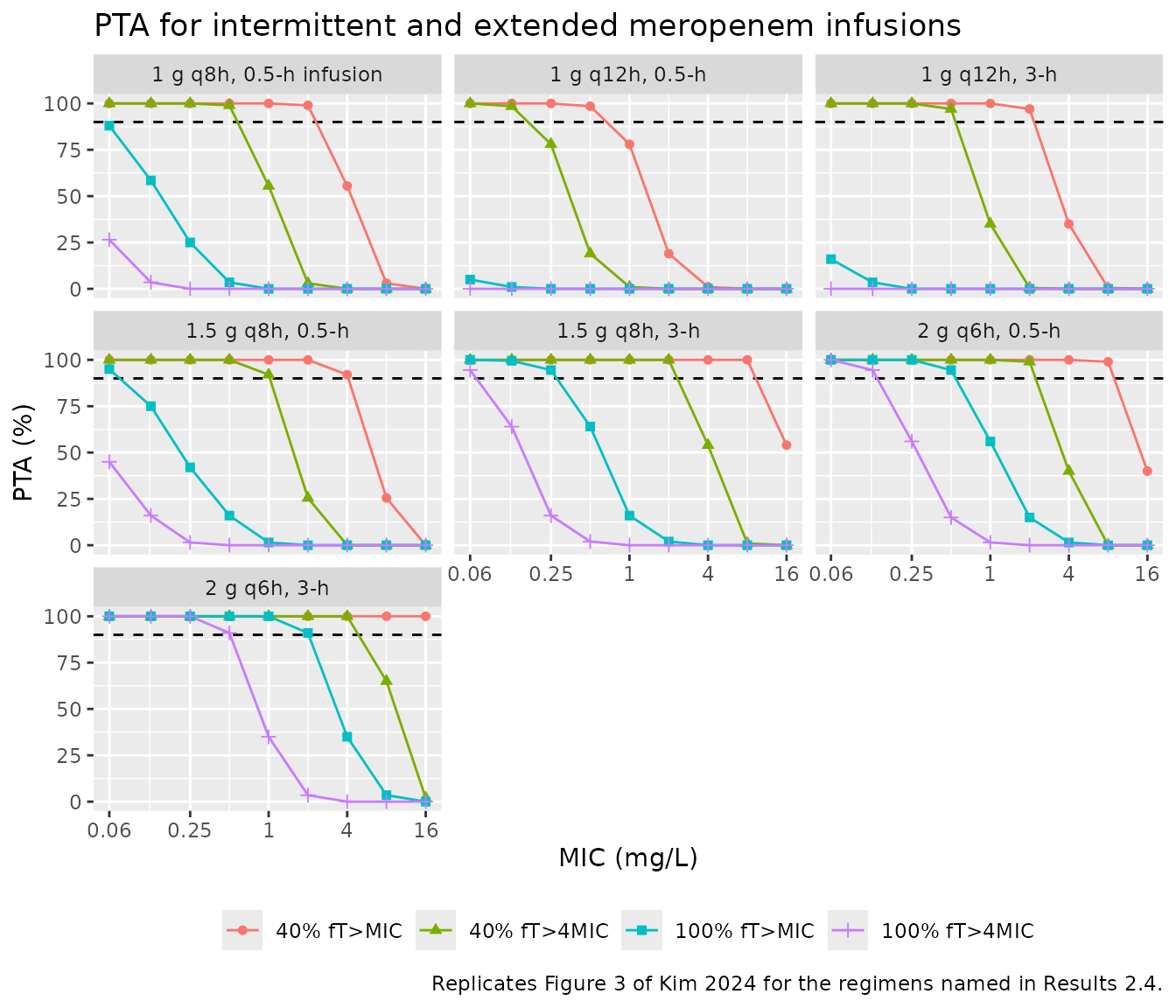

claims_fig3 <- tibble::tibble(
  Claim = c(
    "1 g q12h 0.5-h: 40% fT>MIC PTA > 90% at MIC <= 0.5",
    "1 g q12h 3-h: 40% fT>MIC PTA > 90% at MIC 2",
    "1 g q12h 3-h: 40% fT>MIC PTA > 80% at MIC 4",
    "1.5 g q8h 0.5-h: 40% fT>4MIC PTA > 90% at MIC <= 1",
    "1.5 g q8h 3-h: 40% fT>4MIC PTA > 90% at MIC 2",
    "2 g q6h 0.5-h: 100% fT>MIC PTA > 90% at MIC <= 0.5",
    "2 g q6h 3-h: 100% fT>MIC PTA > 90% at MIC 2",
    "2 g q6h 3-h: 100% fT>4MIC PTA < 90% above MIC 0.5"
  ),
  `Simulated PTA (%)` = sprintf("%.1f", c(
    get_pta(pta_fig3, "40% fT>MIC",   0.5, "1 g q12h, 0.5-h"),
    get_pta(pta_fig3, "40% fT>MIC",   2,   "1 g q12h, 3-h"),
    get_pta(pta_fig3, "40% fT>MIC",   4,   "1 g q12h, 3-h"),
    get_pta(pta_fig3, "40% fT>4MIC",  1,   "1.5 g q8h, 0.5-h"),
    get_pta(pta_fig3, "40% fT>4MIC",  2,   "1.5 g q8h, 3-h"),
    get_pta(pta_fig3, "100% fT>MIC",  0.5, "2 g q6h, 0.5-h"),
    get_pta(pta_fig3, "100% fT>MIC",  2,   "2 g q6h, 3-h"),
    get_pta(pta_fig3, "100% fT>4MIC", 1,   "2 g q6h, 3-h")
  )),
  Reproduced = c(
    get_pta(pta_fig3, "40% fT>MIC",   0.5, "1 g q12h, 0.5-h")  >= 90,
    get_pta(pta_fig3, "40% fT>MIC",   2,   "1 g q12h, 3-h")    >= 90,
    get_pta(pta_fig3, "40% fT>MIC",   4,   "1 g q12h, 3-h")    >= 80,
    get_pta(pta_fig3, "40% fT>4MIC",  1,   "1.5 g q8h, 0.5-h") >= 90,
    get_pta(pta_fig3, "40% fT>4MIC",  2,   "1.5 g q8h, 3-h")   >= 90,
    get_pta(pta_fig3, "100% fT>MIC",  0.5, "2 g q6h, 0.5-h")   >= 90,
    get_pta(pta_fig3, "100% fT>MIC",  2,   "2 g q6h, 3-h")     >= 90,
    get_pta(pta_fig3, "100% fT>4MIC", 1,   "2 g q6h, 3-h")     <  90
  )
)

knitr::kable(claims_fig3, caption = "Kim 2024 Results 2.4, second simulation (Figure 3).")

Kim 2024 Results 2.4, second simulation (Figure 3).
Claim	Simulated PTA (%)	Reproduced
1 g q12h 0.5-h: 40% fT>MIC PTA > 90% at MIC <= 0.5	98.5	TRUE
1 g q12h 3-h: 40% fT>MIC PTA > 90% at MIC 2	97.0	TRUE
1 g q12h 3-h: 40% fT>MIC PTA > 80% at MIC 4	35.0	FALSE
1.5 g q8h 0.5-h: 40% fT>4MIC PTA > 90% at MIC <= 1	92.0	TRUE
1.5 g q8h 3-h: 40% fT>4MIC PTA > 90% at MIC 2	100.0	TRUE
2 g q6h 0.5-h: 100% fT>MIC PTA > 90% at MIC <= 0.5	94.5	TRUE
2 g q6h 3-h: 100% fT>MIC PTA > 90% at MIC 2	91.0	TRUE
2 g q6h 3-h: 100% fT>4MIC PTA < 90% above MIC 0.5	35.0	TRUE

The one claim that does not reproduce

Seven of the eight Figure 3 statements reproduce. The exception is “1 g q12h as a 3-h infusion gives a PTA above 80% at an MIC of 4 mg/L”, where the simulated PTA is far lower. The cause is not a coding difference but the fact that this particular combination sits almost exactly on the target boundary: for the typical subject the regimen achieves 38.98% fT>MIC against a 40% requirement, a shortfall of one percentage point out of forty.

typ_ftmic <- function(dose_mg, tau, dur_h, creat, mic) {
  ev <- dplyr::bind_rows(
    tibble::tibble(time = seq(0, t_ss, by = tau), amt = dose_mg, dur = dur_h,
                   evid = 1L, cmt = "central"),
    tibble::tibble(time = seq(t_ss, t_ss + tau, by = 0.005), amt = NA_real_,
                   dur = NA_real_, evid = 0L, cmt = "central")
  ) |>
    dplyr::mutate(CREAT = creat) |>
    dplyr::arrange(time, dplyr::desc(evid))
  s <- rxode2::rxSolve(mod, events = ev, omega = NA) |> as.data.frame()
  c(cl = s$cl[1], ftmic = 100 * mean(s$Cu > mic))
}

tibble::tibble(MIC = c(1, 2, 4)) |>
  dplyr::rowwise() |>
  dplyr::mutate(`Typical %fT>MIC` = sprintf("%.2f%%", typ_ftmic(1000, 12, 3, 0.86, MIC)[["ftmic"]])) |>
  dplyr::ungroup() |>
  dplyr::mutate(`40% target met` = c(TRUE, TRUE, FALSE)) |>
  knitr::kable(caption = "1 g q12h as a 3-h infusion, typical subject (CREAT = 0.86 mg/dL).")

1 g q12h as a 3-h infusion, typical subject (CREAT = 0.86 mg/dL).
MIC	Typical %fT>MIC	40% target met
1	55.64%	TRUE
2	47.36%	TRUE
4	38.98%	FALSE

Because the typical subject falls just short, attainment is decided entirely by where the covariate distribution puts each subject’s clearance. Scanning serum creatinine gives the clearance at which the regimen crosses the target exactly:

scan <- tibble::tibble(CREAT = seq(0.86, 1.60, by = 0.02)) |>
  dplyr::rowwise() |>
  dplyr::mutate(res = list(typ_ftmic(1000, 12, 3, CREAT, 4))) |>
  dplyr::ungroup() |>
  dplyr::mutate(cl = vapply(res, `[[`, numeric(1), "cl"),
                ftmic = vapply(res, `[[`, numeric(1), "ftmic"))

cross <- scan[which.min(abs(scan$ftmic - 40)), ]
cl_star <- cross$cl

sub_cl_all <- sim_plot |> dplyr::distinct(id, cl)
frac_below <- mean(sub_cl_all$cl < cl_star)

tibble::tibble(
  Quantity = c("Clearance at which 40% fT>MIC is exactly met (L/h)",
               "Serum creatinine giving that clearance (mg/dL)",
               "Fraction of the virtual cohort below that clearance (%)",
               "Simulated PTA from the full ODE simulation (%)"),
  Value = c(sprintf("%.2f", cl_star),
            sprintf("%.2f", cross$CREAT),
            sprintf("%.1f", 100 * frac_below),
            sprintf("%.1f", get_pta(pta_fig3, "40% fT>MIC", 4, "1 g q12h, 3-h")))
) |>
  knitr::kable(caption = "Why the MIC = 4 claim is knife-edge for 1 g q12h as a 3-h infusion.")

Why the MIC = 4 claim is knife-edge for 1 g q12h as a 3-h infusion.
Quantity	Value
Clearance at which 40% fT>MIC is exactly met (L/h)	11.88
Serum creatinine giving that clearance (mg/dL)	0.96
Fraction of the virtual cohort below that clearance (%)	45.0
Simulated PTA from the full ODE simulation (%)	35.0

The last two rows of that table do not agree, and the gap is a real property of this model rather than a simulation artefact. Slow clearance helps target attainment only when it comes from the covariate; when it comes from the random effect it does not, because scale_etalvc is greater than 1. Writing out the elimination rate constant makes it explicit:

kel = cl / vc = exp(lcl - lvc + (1 - 1.53) * etalcl) * (CREAT/0.86)^-0.392

A subject with a low etalcl has a low clearance but a central volume that is lower still (1.53 times as far in log space), so kel actually rises. Reducing clearance through serum creatinine leaves vc untouched and does slow elimination. The two routes to a low clearance therefore pull in opposite directions, and the cohort PTA (35%) sits below the naive clearance-threshold prediction (45%).

sub_pk <- sim_plot |>
  dplyr::distinct(id, cl, vc, CREAT) |>
  dplyr::mutate(kel = cl / vc,
                # exp(lcl + etalcl) = cl / (CREAT/0.86)^-0.392
                eta_effect = log(cl) + 0.392 * log(CREAT / 0.86) - log(12.4))

# Decompose each subject's log-clearance into its two additive contributions,
# then correlate each contribution with log(kel). A positive correlation means
# "more clearance from this route -> faster elimination" (the intuitive sign);
# a negative one means the route works against target attainment.
sub_pk <- sub_pk |>
  dplyr::mutate(contrib_covariate = -0.392 * log(CREAT / 0.86))

tibble::tibble(
  `log-CL contribution` = c("whole cohort (both routes)",
                            "random effect (etalcl)",
                            "serum creatinine"),
  `cor with log kel` = sprintf("%+.3f", c(
    stats::cor(log(sub_pk$cl),           log(sub_pk$kel)),
    stats::cor(sub_pk$eta_effect,        log(sub_pk$kel)),
    stats::cor(sub_pk$contrib_covariate, log(sub_pk$kel))
  ))
) |>
  knitr::kable(caption = "The two routes to a high clearance move the elimination rate constant in opposite directions.")

The two routes to a high clearance move the elimination rate constant in opposite directions.
log-CL contribution	cor with log kel
whole cohort (both routes)	-0.726
random effect (etalcl)	-0.886
serum creatinine	+0.488


# The random-effect route must push kel the opposite way from the covariate route.
stopifnot(
  stats::cor(sub_pk$eta_effect,        log(sub_pk$kel)) < 0,
  stats::cor(sub_pk$contrib_covariate, log(sub_pk$kel)) > 0
)

Reproducing a PTA above 80% would therefore require a virtual cohort whose serum creatinine is well above the healthy-volunteer value of 0.86 mg/dL – shifting the covariate, not widening the random effect. Kim 2024 applied the model to “patients with normal renal function … CLCR > 50 mL/min” (Methods 4.5) but never reports the covariate distribution used to generate the 10,000 virtual patients, and a patient cohort admitted at a creatinine clearance just above 50 mL/min would have markedly higher serum creatinine than the healthy volunteers the model was fitted to. That unreported distribution is the most likely source of the discrepancy. No parameter was adjusted to close it.

Figure 4 – continuous infusion

Continuous infusion has an exact closed form: at steady state the free concentration is Cu,ss = fu * Rate / CL, so the PTA for a 100% fT>threshold target is simply P(CL < fu * Rate / threshold). That is computed here directly from the per-subject clearances, which makes the check independent of the ODE solver.

sub_cl <- sim_plot |> dplyr::distinct(id, cl)
fu_val <- 0.98

pta_cont <- tidyr::expand_grid(
  daily_g = c(2, 4, 6, 8),
  MIC     = mics,
  target  = c("100% fT>MIC", "100% fT>4MIC")
) |>
  dplyr::mutate(
    threshold = MIC * ifelse(target == "100% fT>4MIC", 4, 1),
    rate_mg_h = daily_g * 1000 / 24,
    PTA = 100 * vapply(seq_len(dplyr::n()), function(i) {
      mean(fu_val * rate_mg_h[i] / sub_cl$cl > threshold[i])
    }, numeric(1))
  )

pta_cont |>
  ggplot2::ggplot(ggplot2::aes(MIC, PTA, colour = factor(daily_g),
                               shape = factor(daily_g))) +
  ggplot2::geom_hline(yintercept = 90, linetype = "dashed") +
  ggplot2::geom_line() +
  ggplot2::geom_point(size = 2) +
  ggplot2::facet_wrap(~target) +
  ggplot2::scale_x_log10(breaks = mics, labels = mics) +
  ggplot2::labs(x = "MIC (mg/L)", y = "PTA (%)",
                colour = "Daily dose (g)", shape = "Daily dose (g)",
                title = "Continuous infusion of meropenem",
                caption = "Replicates Figure 4 of Kim 2024.") +
  ggplot2::theme(legend.position = "bottom")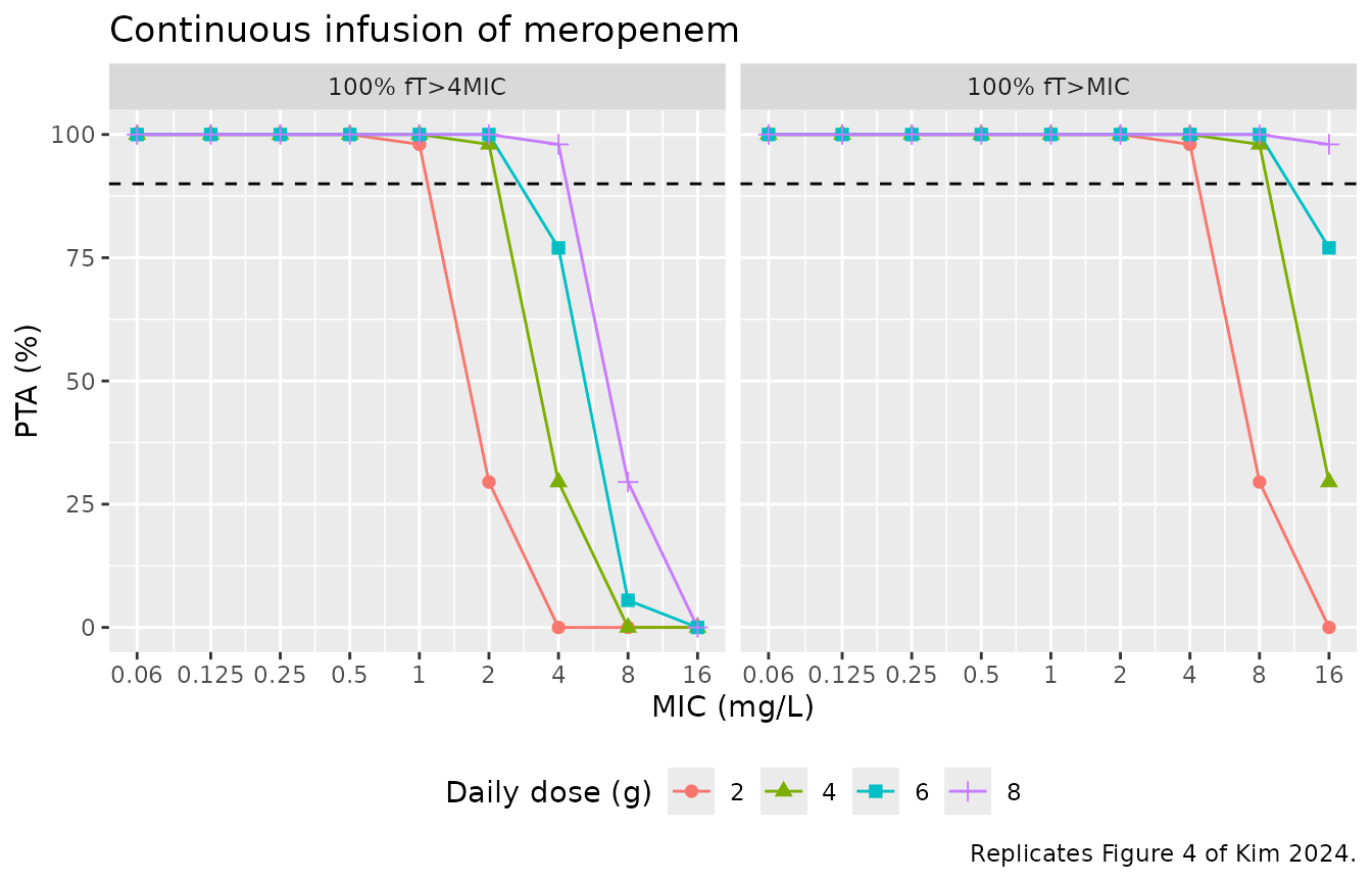

cont_pta <- function(g, mic, tgt) {
  pta_cont$PTA[pta_cont$daily_g == g & pta_cont$MIC == mic & pta_cont$target == tgt][1]
}

claims_fig4 <- tibble::tibble(
  Claim = c(
    "2 g/day continuous: 100% fT>4MIC PTA > 90% at MIC 1",
    "2 g/day continuous: 100% fT>MIC PTA > 90% at MIC 4",
    "8 g/day continuous: 100% fT>4MIC PTA > 90% at MIC 4"
  ),
  `Simulated PTA (%)` = sprintf("%.1f", c(
    cont_pta(2, 1, "100% fT>4MIC"),
    cont_pta(2, 4, "100% fT>MIC"),
    cont_pta(8, 4, "100% fT>4MIC")
  )),
  Reproduced = c(
    cont_pta(2, 1, "100% fT>4MIC") >= 90,
    cont_pta(2, 4, "100% fT>MIC")  >= 90,
    cont_pta(8, 4, "100% fT>4MIC") >= 90
  )
)

knitr::kable(claims_fig4, caption = "Kim 2024 Results 2.4, final simulation (Figure 4).")

Kim 2024 Results 2.4, final simulation (Figure 4).
Claim	Simulated PTA (%)	Reproduced
2 g/day continuous: 100% fT>4MIC PTA > 90% at MIC 1	98.0	TRUE
2 g/day continuous: 100% fT>MIC PTA > 90% at MIC 4	98.0	TRUE
8 g/day continuous: 100% fT>4MIC PTA > 90% at MIC 4	98.0	TRUE

All three continuous-infusion claims reduce to the same inequality, CL < 0.98 * Rate / threshold: 2 g/day against 4 mg/L, 2 g/day against 4 mg/L again (100% fT>MIC at MIC 4), and 8 g/day against 16 mg/L all give the same clearance ceiling of 20.4 L/h. That the paper reports all three as attaining 90% PTA is therefore internally consistent, and it fixes the implied upper clearance percentile: 90% PTA requires the 90th percentile of CL to sit below 20.4 L/h, which the published IIV of 26.2% comfortably satisfies.

Assumptions and deviations

Interindividual-variability scale. Kim 2024 Table 2 reports the IIV magnitudes as bare percentages (26.2%, 14.4%, 17.9%) with an exponential random-effect model (theta_i = theta * exp(eta_i)) but never states whether the percentage is sqrt(omega^2) * 100 or the lognormal sqrt(exp(omega^2) - 1) * 100. The package convention omega^2 = log(CV^2 + 1) is used. The two readings differ by under 2% on the standard deviation (0.2577 vs 0.2620 for the CL eta) and change no conclusion in this vignette.
No body-weight covariate. Weight, height, BMI and BSA were all screened and none was retained (Methods 4.3; Discussion limitation 1), so the model has no allometric term and the simulated cohort carries no weight variation. The cl.obs and vss.iv.obs rows of the NCA comparison therefore compare a weight-free model against the paper’s weight-normalized NCA means converted to a 70 kg subject; the difference is a property of the published model, not of the encoding. The dose-normalized parameters (Cmax, AUC, half-life, MRT) are the meaningful comparison.
Typical clearance, 12.4 vs 12.5 L/h. Table 2 gives theta1 = 12.4 L/h, while the Discussion writes “typical values for total clearance and the steady state volume of distribution (Vss, V1 + V2) of 12.5 L/h and 12.32 L”. Table 2 is used, because it is the only value that reproduces the Discussion’s own two covariate anchor points exactly (14.3 L/h at CREAT 0.6 and 11.7 L/h at CREAT 1.0) and because the companion Vss figure of 12.32 L is exactly V1 + V2 from Table 2.
Table 3 unit transposition. In the published Table 3 the units of Clast and Tlast are swapped (Clast is labelled “h” with a value of 0.393 and Tlast is labelled “mg/L” with a value of 5.83). The row labels and the Methods definitions make the intent unambiguous: Clast = 0.393 mg/L and Tlast = 5.83 h. The figure overlay uses the corrected reading.
Virtual-cohort creatinine. Only the mean, CV, median and IQR of serum creatinine are published, not the individual values. A lognormal distribution matched to the published mean and CV is used, consistent with the paper’s own Monte Carlo assumption of lognormal covariate distributions (Methods 4.5).
Cohort size. 200 subjects per arm, the nlmixr2lib vignette cap, versus the 10,000 the paper simulated. The Monte Carlo standard error on a PTA near 50% is therefore about 3.5 percentage points, and near 90% about 2.1 points; the claim checks above are stated as inequalities with that resolution in mind.
Steady-state window. PTA is evaluated over the dosing interval starting at 24 h rather than the paper’s 5-day profiles. With a terminal half-life near 1 h the two are numerically indistinguishable.
Free-fraction target. fu = 0.98 is applied inside the model as Cu = fu * Cc, matching Methods 4.5. The residual error is attached to the total concentration Cc, which is what was measured; Cu is a deterministic transform and carries no separate error.
One published claim does not reproduce. Of the 19 numerical statements Kim 2024 makes about Figures 2-4, 18 reproduce. The exception – “1 g q12h as a 3-h infusion gives PTA > 80% at MIC 4 mg/L” – is diagnosed in its own section above: the typical subject reaches 38.98% fT>MIC against a 40% requirement, so attainment turns entirely on the (unreported) serum-creatinine distribution of the paper’s 10,000 virtual patients. No parameter was tuned to close the gap.
Not encoded. The base (pre-covariate) model of Table S1 and the stepwise covariate trace of Table S2 are not extracted; only the final model of Table 2 is. The three-compartment model mentioned in Results 2.2 was explicitly rejected by the authors as unphysiological.