Midazolam CRRT circuit (McKnite 2026)
Source:vignettes/articles/McKnite_2026_midazolam_crrt.Rmd
McKnite_2026_midazolam_crrt.RmdModel and source
Citation: McKnite AM, Hamadeh A, Hunt JP, Green DJ, Imburgia C, Whelan A, Hudson R, Chevalier A, Mathis CL, Yang MJ, Dwyer JP, Edginton A, Watt KM. Midazolam Dosing During CRRT: A Combined Ex Vivo and Physiologically-Based Pharmacokinetic Approach. CPT Pharmacometrics Syst Pharmacol. 2026;15:e70240. doi:10.1002/psp4.70240. PMCID: PMC13274749. Circuit structure and the ex vivo prescription: Methods 2.5. Optimized Michaelis-Menten constants: Results 3.3. Flow / hematocrit derivations (Equations 1-6) and mass transfers (Equations 7-11): Supporting Information Appendix S1. Membrane diffusion coefficient, the unrounded Vmax, the plasma / red-cell exchange terms and the red-cell partition coefficient come from the authors’ deposited MoBi 10.0 project (Appendix S1, ‘PSP-2025-0082-s02’); see the per-parameter comments and the vignette source-trace table.
Description: Ex vivo (extracorporeal continuous renal replacement therapy circuit). Mechanistic six-state model of midazolam disposition in a Baxter PrisMax CRRT circuit fitted to closed-loop ex vivo data: a blood reservoir split into plasma and red-cell sub-compartments feeds a hemofilter that is likewise split into plasma and red-cell sub-compartments, which exchanges drug with the filter dialysate by diffusion across the membrane and by convection with the filtrate, and the dialysate drains to effluent waste. Circuit adsorption (plus any filter clearance and degradation not otherwise accounted for) is a saturable Michaelis-Menten sink acting on the filter plasma and red-cell states. Flow and hematocrit derivations are Equations 1-6 and the mass transfers Equations 7-11 of Supplement S1. The paper’s whole-body child CRRT-PBPK model, which grafts this circuit onto a 17-compartment PK-Sim/MoBi pediatric model, is NOT reproduced here; only the transferable circuit module is.
Article: https://doi.org/10.1002/psp4.70240
Open-access full text: https://europepmc.org/article/MED/PMC13274749
Supporting Information (Appendix S1, holding Equations 1-11, Tables S1-S6 and the authors’ MoBi 10.0 project file): https://doi.org/10.1002/psp4.70240
What this file is, and what it is not
McKnite and colleagues built five things:
| # | Model | Implementation | In this file? |
|---|---|---|---|
| 1 | Adult whole-body midazolam PBPK (17 compartments) | PK-Sim | no |
| 2 | Child whole-body PBPK with CYP3A4 ontogeny | PK-Sim | no |
| 3 | Preterm PBPK adding CYP3A7 | PK-Sim | no |
| 4 | Ex vivo CRRT circuit (Methods 2.5, Figure 1A) | MoBi | yes |
| 5 | Child CRRT-PBPK (4 grafted onto 2) | PK-Sim + MoBi | no |
Models 1, 2, 3 and 5 are whole-body Open Systems Pharmacology models. The authors’ deposited MoBi project resolves to 179 physical containers, 255 neighborhoods and 3245 structural parameters, with all eleven gastrointestinal lumen segments, liver zonation, mucosa, saliva and gallbladder present. Their parameter values are recoverable, but their size puts them outside what a single nlmixr2lib model file should hold; they are recorded as a deferred platform port.
Model 4 is a different object. It is ~6 states, its rate laws are
printed verbatim in Appendix S1 as Equations 1-11, its two fitted
constants are printed in Results 3.3, and the authors offer it as the
paper’s transferable contribution: “The CRRT compartment can be
easily adapted to other drugs using ex vivo experiments to determine
drug clearance by the circuit.” That is what
McKnite_2026_midazolam_crrt packages.
The compartment names circuit_plasma,
circuit_rbc, circuit_dialysate,
circuit_effluent, reservoir_plasma and
reservoir_rbc are a new canonical family registered with
this model (see inst/references/compartment-names.md). They
are deliberately modality-neutral so that a later ECMO oxygenator,
apheresis column or haemoperfusion cartridge reuses them. Note that
Kim_2026_midazolam_ecmo, the nearest existing model,
carries an extracorporeal circuit only as a covariate on clearance
(Q_ECMO) and has no circuit states at all; this is the
library’s first structural extracorporeal circuit.
Population
The circuit model was fitted to an ex vivo bench system, not to patients: a Baxter PrisMax platform running an HF1000 hemofilter in a closed loop against a 600 mL blood reservoir at hematocrit 0.30, those two values being the means across three replicate experiments (Methods 2.5). The CRRT prescription was blood flow 80 mL/min, dialysate 400 mL/h, pre-blood pump 300 mL/h, replacement fluid 100 mL/h and no patient fluid removal, i.e. continuous venovenous hemodiafiltration. Midazolam was simulated at a circuit concentration of 0.15 mg/L.
The concentration-time data the two Michaelis-Menten constants were optimized against come from a previously published ex vivo study by the same group (reference 13 of the source paper) and are not reproduced in this paper, so the blood source and the exact albumin concentration of those circuits are documented there rather than here.
Downstream, the paper applies the circuit to three children aged 12, 22 and 72 months (Table S2) and to five 1000-subject age-stratified virtual populations from neonates to adolescents (Tables S4 and S5). Those simulations exercise the whole-body model this module was grafted onto. The per-age-group CRRT prescriptions from Table S4, however, are pure circuit configuration, and they are used below to characterise the module across the paper’s own clinical settings.
str(readModelDb("McKnite_2026_midazolam_crrt")()$population)
#> List of 11
#>  $ species      : chr "ex vivo (closed-loop extracorporeal CRRT circuit primed with whole blood)"
#>  $ n_subjects   : int NA
#>  $ n_studies    : int 1
#>  $ system       : chr "Baxter PrisMax continuous renal replacement therapy platform running an HF1000 hemofilter (Baxter Healthcare, D"| __truncated__
#>  $ n_replicates : int 3
#>  $ hematocrit   : chr "0.30 (mean of three ex vivo replicates)"
#>  $ modality     : chr "continuous venovenous hemodiafiltration (CVVHDF)"
#>  $ prescription : chr "Blood flow 80 mL/min; dialysate flow 400 mL/h; pre-blood pump 300 mL/h; replacement fluid 100 mL/h; patient flu"| __truncated__
#>  $ dose_range   : chr "single spike to a circuit concentration of 0.15 mg/L"
#>  $ disease_state: chr "not applicable (ex vivo)"
#>  $ notes        : chr "Methods 2.5 and Figure 1A. The ex vivo concentration data the Michaelis-Menten constants were optimized against"| __truncated__
Source trace
Per-parameter origin is recorded as an in-file comment beside each
ini() entry in
inst/modeldb/specificDrugs/McKnite_2026_midazolam_crrt.R.
Collected here for review.
| Equation / parameter | Value | Source location |
|---|---|---|
qfil = qpbp + qrep + qpfr |
n/a | Appendix S1 Equation 1 |
qeff = qdia + qfil |
n/a | Appendix S1 Equation 2 |
(Q_PR, total fluid removal) |
not carried | Appendix S1 Equation 3; a reporting quantity that enters no mass transfer |
qret = qbfr - qrep - qpfr |
n/a | Appendix S1 Equation 4 |
hctin = hct * qbfr / (qbfr + qpbp) |
n/a | Appendix S1 Equation 5 |
hctout = hct * qbfr / qret |
n/a | Appendix S1 Equation 6 |
hctfil = (hctin + hctout) / 2 |
n/a | Not printed; the filter plasma / red-cell volume split stored in the deposited MoBi project |
| red-cell delivery / return flux | n/a | Appendix S1 Equation 7 (Q_BFR * HCT * C_rbc); the
return leg’s Q_RET * HCT_OUT form is from the deposited
project, which is what Equations 4 and 6 exist to supply |
| plasma delivery / return flux | n/a | Appendix S1 Equation 8 (Q_BFR * (1 - HCT) * C_pls) |
jdiff = (D * SA / h) * (fu * C_pls - C_dia) |
n/a | Appendix S1 Equation 9 |
jconv = fu * qfil * C_pls |
n/a | Appendix S1 Equation 10 |
jeff = C_dia * qeff |
n/a | Appendix S1 Equation 11 |
saturable circuit loss vmaxcrrt * C / (C + kmcrrt)
|
n/a | Appendix S1 closing paragraph (“the elimination rate constant
included drug adsorption, clearance by the dialysis filter and, if
present, drug degradation”); rate law from the deposited project’s
MidazolamDegradation reaction |
plasma / red-cell exchange
PS * (C_pls - C_rbc / krbc)
|
n/a | Not printed; the deposited project’s
PassiveDiffusionPl2RBC transport |
qbfr |
4.8 L/h | Methods 2.5, “blood flow rate, 80 mL/min” |
qdia |
0.4 L/h | Methods 2.5, “dialysate flow rate, 400 mL/min” – unit typo, see Errata |
qpbp |
0.3 L/h | Methods 2.5, “pre-blood pump, 300 mL/h” |
qrep |
0.1 L/h | Methods 2.5, “replacement fluids, 100 mL/h” |
qpfr |
0 L/h | Methods 2.5, “patient fluid removal, 0 mL/h” |
hct |
0.30 | Methods 2.5, mean of three ex vivo replicates |
vreservoir |
0.600 L | Methods 2.5, “a reservoir volume of 600 mL” |
vfilter |
0.165 L | Methods 2.5, “filter volume 165 mL”; equals the HF1000 circuit blood volume in Table S3 |
vdialysate |
0.0591 L | Methods 2.5, “dialysate volume 59.1 mL” |
safilter |
120 dm^2 | Methods 2.5, “surface area 1.2 m2”; Table S3 lists 1.1 m2, see Errata |
thfilter |
5e-4 dm | Methods 2.5, “membrane thickness 50 um”; Table S3 lists 50 um for every filter |
dfilter |
0.594 dm^2/h |
Not printed. Deposited MoBi project, HF1000
MembraneDiffusionCoefficient = 0.0099 dm^2/min |
fu |
0.02 | Table 1, optimized fraction unbound 2.0% |
krbc |
0.2492 |
Not printed. Evaluated from the deposited project’s
own K_rbc formula; see Errata |
permrbc |
0.3004 dm/h |
Not printed. Evaluated from the deposited project’s
own P formula; see Errata |
satovrbc |
1.002e6 1/dm |
Not printed. Deposited project,
Surface/Volume ratio (blood cells) 167000 1/cm times the
OSP accessibility factor 0.6 |
vmaxcrrt |
0.047888 mg/h | Results 3.3, “V max of 0.002 L/min”; unrounded 0.00245 from the deposited project, converted with MW 325.77 g/mol (Table 1) |
kmcrrt |
0.358347 mg/L | Results 3.3, “a final K m of 1100 pmol/mL”, converted with MW 325.77 g/mol |
propSd |
fixed 0 | No residual-error model reported anywhere; see Errata |
Circuit configurations
There is no virtual cohort here: the model has no between-subject variability, no residual error and no covariates, because the source is a deterministic mechanistic fit to a bench apparatus. What varies instead is the circuit configuration. Six arms are simulated: the ex vivo circuit the model was fitted to, and the five per-age-group clinical CRRT prescriptions of Table S4, each with the filter geometry Table S3 gives for its filter type.
# Table S3, filter parameters. Membrane thickness is 50 um for every filter.
filters <- tibble::tribble(
  ~filter,  ~sa_m2, ~circuit_ml,
  "HF20",      0.2,          58,
  "HF1000",    1.1,         165,
  "M60",       0.6,          93,
  "M100",      0.9,         152,
  "ST150",     1.5,         189
)

# Table S4, virtual-population CRRT prescriptions; plus the ex vivo circuit of
# Methods 2.5 as the reference arm. `qdia_mlh` for the ex vivo arm is the
# typo-corrected 400 mL/h (see Errata). `wt_kg` is the Table S4 weight, used
# only to express circuit clearance per kilogram.
arms <- tibble::tribble(
  ~arm,          ~filter,  ~bfr_mlmin, ~qdia_mlh, ~qpbp_mlh, ~qrep_mlh, ~qpfr_mlh, ~wt_kg,
  "Ex vivo",     "HF1000",         80,       400,       300,       100,         0,     NA,
  "Neonatal",    "HF20",           20,       900,         0,         0,       120,    3.5,
  "Infant",      "HF20",           30,       500,        68,       100,        55,    5.1,
  "Child",       "M60",            90,       800,       170,       100,       200,   14.0,
  "School age",  "M100",          120,      1300,       270,       100,       270,   29.7,
  "Adolescent",  "ST150",         150,      2000,       310,       100,       250,   56.6
)

arms <- arms |>
  dplyr::left_join(filters, by = "filter") |>
  # The ex vivo arm takes its filter geometry from Methods 2.5 rather than from
  # Table S3, because those are the numbers the ex vivo circuit was actually
  # parameterised with: surface area 1.2 m2 (Table S3 lists 1.1 m2 for the
  # HF1000, see Errata) and a measured dialysate volume of 59.1 mL. Everything
  # else follows Table S3.
  dplyr::mutate(
    sa_m2 = ifelse(arm == "Ex vivo", 1.2, sa_m2),
    vdia_ml = ifelse(arm == "Ex vivo", 59.1, NA_real_),
    id = seq_len(dplyr::n()),
    # Flows to L/h. Blood flow is printed in mL/min, everything else in mL/h.
    qbfr = bfr_mlmin * 0.06,
    qdia = qdia_mlh / 1000,
    qpbp = qpbp_mlh / 1000,
    qrep = qrep_mlh / 1000,
    qpfr = qpfr_mlh / 1000,
    # Filter geometry. The membrane surface area is printed in m^2 and the
    # model wants dm^2; the blood-side volume is the Table S3 circuit blood
    # volume, matching what Methods 2.5 used for the HF1000.
    safilter = sa_m2 * 100,
    vfilter = circuit_ml / 1000,
    # ASSUMPTION for the five clinical arms. Table S3 does not tabulate a
    # dialysate-side volume for any filter; Methods 2.5 gives it only for the
    # HF1000 (59.1 mL, "equivalent to HF1000 filter prime volume"). Scaled here
    # with membrane surface area from that single anchor. The sensitivity check
    # below shows the model output is insensitive to this choice, because the
    # membrane permeability-surface product is five orders of magnitude larger
    # than the effluent flow.
    vdialysate = dplyr::coalesce(vdia_ml, 59.1 * sa_m2 / 1.2) / 1000
  )

knitr::kable(
  arms |>
    dplyr::select(arm, filter, qbfr, qdia, qpbp, qrep, qpfr, safilter, vfilter, vdialysate) |>
    dplyr::rename(
      "Arm" = arm, "Filter" = filter,
      "Q_BFR (L/h)" = qbfr, "Q_DIA (L/h)" = qdia, "Q_PBP (L/h)" = qpbp,
      "Q_REP (L/h)" = qrep, "Q_PFR (L/h)" = qpfr,
      "SA (dm2)" = safilter, "V filter (L)" = vfilter, "V dialysate (L)" = vdialysate
    ),
  digits = 4,
  caption = "Circuit configurations. Ex vivo arm from Methods 2.5; the five clinical arms from Table S4 with filter geometry from Table S3."
)| Arm | Filter | Q_BFR (L/h) | Q_DIA (L/h) | Q_PBP (L/h) | Q_REP (L/h) | Q_PFR (L/h) | SA (dm2) | V filter (L) | V dialysate (L) |
|---|---|---|---|---|---|---|---|---|---|
| Ex vivo | HF1000 | 4.8 | 0.4 | 0.300 | 0.1 | 0.000 | 120 | 0.165 | 0.0591 |
| Neonatal | HF20 | 1.2 | 0.9 | 0.000 | 0.0 | 0.120 | 20 | 0.058 | 0.0099 |
| Infant | HF20 | 1.8 | 0.5 | 0.068 | 0.1 | 0.055 | 20 | 0.058 | 0.0099 |
| Child | M60 | 5.4 | 0.8 | 0.170 | 0.1 | 0.200 | 60 | 0.093 | 0.0296 |
| School age | M100 | 7.2 | 1.3 | 0.270 | 0.1 | 0.270 | 90 | 0.152 | 0.0443 |
| Adolescent | ST150 | 9.0 | 2.0 | 0.310 | 0.1 | 0.250 | 150 | 0.189 | 0.0739 |
Every arm keeps the ex vivo reservoir (600 mL at hematocrit 0.30).
For the five clinical arms the reservoir is a numerical device, not a
claim about a patient’s blood volume: the quantity extracted from those
arms is the circuit clearance Dose / AUCinf, which is
independent of the reservoir volume, so only the time scale of
those curves depends on it and no time-course prediction is read off
them.
Simulation
mod <- readModelDb("McKnite_2026_midazolam_crrt")

# Equilibrium split of a reservoir dose between the plasma and red-cell states,
# so the profile starts already equilibrated instead of spiking at t = 0.
hct0 <- 0.30
krbc0 <- 0.2492
f_pls <- (1 - hct0) / ((1 - hct0) + hct0 * krbc0)

# Two doses: the ex vivo spike (0.15 mg/L over the 600 mL reservoir) and a
# 1000-fold lower tracer dose that sits deep in the linear regime of the
# Michaelis-Menten sink, where the closed-form clearance below applies.
dose_exvivo <- 0.15 * 0.600
dose_tracer <- dose_exvivo / 1000

# Fine early grid resolves the redistribution into the filter; coarser later.
obs_times <- sort(unique(c(seq(0, 2, by = 0.02), seq(2, 24, by = 0.1))))

make_events <- function(dose, id) {
  dplyr::bind_rows(
    tibble::tibble(time = 0, amt = dose * f_pls,
                   cmt = "reservoir_plasma", evid = 1L),
    tibble::tibble(time = 0, amt = dose * (1 - f_pls),
                   cmt = "reservoir_rbc", evid = 1L),
    # Observations sit on an ODE STATE, never on the algebraic observable
    # `Cc`; rxode2 returns Cc as a column regardless.
    tibble::tibble(time = obs_times, amt = NA_real_,
                   cmt = "reservoir_plasma", evid = 0L)
  ) |>
    dplyr::mutate(id = id) |>
    dplyr::arrange(time, dplyr::desc(evid))
}

# The circuit prescription and filter geometry are `ini()` parameters, not
# covariates, so they are overridden per arm through `params =` -- an event
# table column of the same name would be silently ignored. One arm per solve;
# six single-subject solves are far cheaper than the alternative.
solve_arms <- function(dose, id_offset = 0L, extra = NULL, arm_tbl = arms) {
  out <- vector("list", nrow(arm_tbl))
  for (i in seq_len(nrow(arm_tbl))) {
    p <- c(
      qbfr = arm_tbl$qbfr[i], qdia = arm_tbl$qdia[i], qpbp = arm_tbl$qpbp[i],
      qrep = arm_tbl$qrep[i], qpfr = arm_tbl$qpfr[i],
      safilter = arm_tbl$safilter[i], vfilter = arm_tbl$vfilter[i],
      vdialysate = arm_tbl$vdialysate[i]
    )
    if (!is.null(extra)) p[names(extra)] <- extra
    id_i <- id_offset + i
    out[[i]] <- rxode2::rxSolve(
      mod, events = make_events(dose, id_i), params = p,
      returnType = "data.frame"
    )
    out[[i]]$id <- id_i
    out[[i]]$arm <- arm_tbl$arm[i]
  }
  dplyr::bind_rows(out)
}

sim_exvivo <- solve_arms(dose_exvivo, id_offset = 0L)
sim_tracer <- solve_arms(dose_tracer, id_offset = 100L)

ev_exvivo <- dplyr::bind_rows(lapply(seq_len(nrow(arms)), function(i) {
  make_events(dose_exvivo, i) |> dplyr::mutate(arm = arms$arm[i])
}))
ev_tracer <- dplyr::bind_rows(lapply(seq_len(nrow(arms)), function(i) {
  make_events(dose_tracer, 100L + i) |> dplyr::mutate(arm = arms$arm[i])
}))

# Disjoint IDs across the two event tables (cheap regression guard).
stopifnot(length(intersect(unique(ev_exvivo$id), unique(ev_tracer$id))) == 0L)

# Solver noise in a far tail would break the PKNCA log-linear fit.
stopifnot(all(sim_exvivo$Cc >= 0), all(sim_tracer$Cc >= 0))
Structural gates
The circuit module has no stochastic component, so every check below is exact and the tolerances are set to the numerical accuracy actually achieved rather than to a cohort spread.
Equations 1-6 reproduce from the model’s own parameters
flows <- arms |>
  dplyr::mutate(
    qfil = qpbp + qrep + qpfr,                 # Eq 1
    qeff = qdia + qfil,                        # Eq 2
    qret = qbfr - qrep - qpfr,                 # Eq 4
    hctin = hct0 * qbfr / (qbfr + qpbp),       # Eq 5
    hctout = hct0 * qbfr / qret                # Eq 6
  )

# Every derived flow must be strictly positive: a prescription whose
# replacement plus removal exceeds the blood flow is not deliverable, and a
# non-positive Q_RET would make Equation 6 diverge.
stopifnot(all(flows$qfil > 0), all(flows$qeff > 0), all(flows$qret > 0))
# Dilution by the pre-blood pump must lower the pre-filter hematocrit, and
# removal of plasma water must raise it again on the way out.
stopifnot(all(flows$hctin <= hct0 + 1e-12),
          all(flows$hctout >= hct0 - 1e-12))

knitr::kable(
  flows |>
    dplyr::select(arm, qfil, qeff, qret, hctin, hctout) |>
    dplyr::rename("Arm" = arm, "Q_FIL (L/h)" = qfil, "Q_EFF (L/h)" = qeff,
                  "Q_RET (L/h)" = qret, "HCT_pre" = hctin, "HCT_post" = hctout),
  digits = 4,
  caption = "Derived circuit flows and hematocrits (Appendix S1 Equations 1, 2, 4, 5, 6)."
)| Arm | Q_FIL (L/h) | Q_EFF (L/h) | Q_RET (L/h) | HCT_pre | HCT_post |
|---|---|---|---|---|---|
| Ex vivo | 0.400 | 0.800 | 4.700 | 0.2824 | 0.3064 |
| Neonatal | 0.120 | 1.020 | 1.080 | 0.3000 | 0.3333 |
| Infant | 0.223 | 0.723 | 1.645 | 0.2891 | 0.3283 |
| Child | 0.470 | 1.270 | 5.100 | 0.2908 | 0.3176 |
| School age | 0.640 | 1.940 | 6.830 | 0.2892 | 0.3163 |
| Adolescent | 0.660 | 2.660 | 8.650 | 0.2900 | 0.3121 |
Mass balance: only adsorption removes drug from the system
With vmaxcrrt set to zero the circuit becomes a closed
system – the effluent compartment is a state, not a sink – so total drug
must be conserved exactly. This is the strongest available check on the
sign and pairing of all twelve flux terms: a single flux written into
one compartment but not out of its partner would show up here
immediately.
states <- c("reservoir_plasma", "reservoir_rbc", "circuit_plasma",
            "circuit_rbc", "circuit_dialysate", "circuit_effluent")

sim_noads <- solve_arms(dose_exvivo, id_offset = 200L,
                        extra = c(vmaxcrrt = 0))
total_noads <- rowSums(sim_noads[, states])
rel_err <- abs(total_noads / dose_exvivo - 1)
cat(sprintf("worst relative mass-balance error with adsorption off: %.3g\n",
            max(rel_err)))
#> worst relative mass-balance error with adsorption off: 8.88e-15
stopifnot(max(rel_err) < 1e-6)
Plasma and red cells reach the partition ratio exactly
late <- sim_exvivo |>
  dplyr::filter(arm == "Ex vivo", time > 1) |>
  dplyr::mutate(
    ratio = (reservoir_rbc / (0.600 * hct0)) /
      (reservoir_plasma / (0.600 * (1 - hct0)))
  )
cat(sprintf("reservoir red-cell / plasma concentration ratio: %.6f (krbc = %.4f)\n",
            mean(late$ratio), krbc0))
#> reservoir red-cell / plasma concentration ratio: 0.249202 (krbc = 0.2492)
stopifnot(max(abs(late$ratio / krbc0 - 1)) < 1e-3)
The dialysate tracks the unbound plasma concentration
The membrane permeability-surface product D * SA / h is
142560 L/h for the HF1000, five orders of magnitude larger than the
effluent flow, so the dialysate compartment sits at quasi-equilibrium
with fu times the filter plasma concentration. This is why
the assumed per-filter dialysate volumes above cannot matter.
xv <- arms[arms$arm == "Ex vivo", ]
hctfil_xv <- 0.5 * (hct0 * xv$qbfr / (xv$qbfr + xv$qpbp) +
                      hct0 * xv$qbfr / (xv$qbfr - xv$qrep - xv$qpfr))

dia <- sim_exvivo |>
  dplyr::filter(arm == "Ex vivo", time > 0.1) |>
  dplyr::mutate(
    c_dia = circuit_dialysate / xv$vdialysate,
    c_fil_pls_unbound = 0.02 * circuit_plasma /
      (xv$vfilter * (1 - hctfil_xv))
  )
# Realised worst deviation 2.9e-6 across the whole 24 h window: the quasi-
# equilibrium is essentially exact, as predicted by
# C_dia / (fu * C_pls) = (K + Q_FIL) / (K + Q_EFF) with K = D * SA / h.
cat(sprintf("worst |C_dialysate / (fu * C_filter_plasma) - 1|: %.3g\n",
            max(abs(dia$c_dia / dia$c_fil_pls_unbound - 1))))
#> worst |C_dialysate / (fu * C_filter_plasma) - 1|: 2.9e-06
stopifnot(max(abs(dia$c_dia / dia$c_fil_pls_unbound - 1)) < 1e-3)

# Because the dialysate sits at that equilibrium, its volume enters the model
# in exactly one way: as an extra distribution volume of size
# `vdialysate * fu`. Nothing else about the circuit depends on it. At the
# sourced value that volume is a fifth of a percent of the system total, so the
# per-filter scaling assumed for the clinical arms cannot matter; the
# clearance-level sensitivity is quantified after the PKNCA section.
v_dia_eq <- xv$vdialysate * 0.02
v_system <- 0.600 * (1 - hct0) + 0.600 * hct0 * krbc0 +
  xv$vfilter * (1 - hctfil_xv) + xv$vfilter * hctfil_xv * krbc0 + v_dia_eq
cat(sprintf("dialysate plasma-equivalent volume %.5g L of %.5g L total (%.3g%%)\n",
            v_dia_eq, v_system, 100 * v_dia_eq / v_system))
#> dialysate plasma-equivalent volume 0.001182 L of 0.59457 L total (0.199%)
stopifnot(v_dia_eq / v_system < 0.005)
PKNCA
The paper reports no NCA parameters for the ex vivo circuit, so there
is no published Cmax / AUC table to place beside these numbers and
nlmixr2lib::ncaComparisonTable() is not used. PKNCA is used
instead to obtain AUCinf per arm, which converts into the
circuit clearance Dose / AUCinf – the quantity that
is checkable, both against a closed form derived from Equations
7-11 and against the paper’s printed pediatric clearance range.
run_nca <- function(sim, ev, dose) {
  conc <- sim |>
    dplyr::filter(!is.na(Cc)) |>
    dplyr::select(id, time, Cc, arm)

  # Guarantee a time-zero row per (id, arm). Never filter on `time > 0` or
  # `Cc > 0`: that drops the row PKNCA anchors AUC0-* on.
  conc <- dplyr::bind_rows(
    conc,
    conc |> dplyr::distinct(id, arm) |> dplyr::mutate(time = 0, Cc = 0)
  ) |>
    dplyr::distinct(id, arm, time, .keep_all = TRUE) |>
    dplyr::arrange(id, arm, time)

  conc_obj <- PKNCA::PKNCAconc(conc, Cc ~ time | arm + id)

  # One dose row per subject: the two dosing events at t = 0 are the plasma /
  # red-cell split of a single spike, so PKNCA sees their total.
  dose_df <- ev |>
    dplyr::filter(evid == 1L) |>
    dplyr::group_by(id, arm) |>
    dplyr::summarise(time = 0, amt = sum(amt), .groups = "drop")
  dose_obj <- PKNCA::PKNCAdose(dose_df, amt ~ time | arm + id)

  intervals <- data.frame(
    start = 0, end = Inf,
    cmax = TRUE, tmax = TRUE, aucinf.obs = TRUE, half.life = TRUE,
    cl.obs = TRUE
  )

  res <- PKNCA::pk.nca(PKNCA::PKNCAdata(conc_obj, dose_obj,
                                        intervals = intervals))
  as.data.frame(res) |>
    dplyr::select(arm, PPTESTCD, PPORRES) |>
    tidyr::pivot_wider(names_from = PPTESTCD, values_from = PPORRES)
}

nca_exvivo <- run_nca(sim_exvivo, ev_exvivo, dose_exvivo)
nca_tracer <- run_nca(sim_tracer, ev_tracer, dose_tracer)

knitr::kable(
  nca_exvivo |>
    dplyr::select(arm, cmax, tmax, aucinf.obs, half.life, cl.obs) |>
    dplyr::rename("Arm" = arm, "Cmax (ug/mL)" = cmax, "Tmax (h)" = tmax,
                  "AUC0-inf (ug*h/mL)" = aucinf.obs, "t1/2 (h)" = half.life,
                  "Circuit CL (L/h)" = cl.obs),
  digits = 4,
  caption = "Non-compartmental summary at the ex vivo dose (0.15 mg/L over the reservoir), by circuit configuration."
)| Arm | Cmax (ug/mL) | Tmax (h) | AUC0-inf (ug*h/mL) | t1/2 (h) | Circuit CL (L/h) |
|---|---|---|---|---|---|
| Adolescent | 0.1936 | 0 | 0.4495 | 1.9126 | 0.2002 |
| Child | 0.1936 | 0 | 0.5283 | 1.9046 | 0.1703 |
| Ex vivo | 0.1936 | 0 | 0.5771 | 2.3059 | 0.1560 |
| Infant | 0.1936 | 0 | 0.5867 | 1.9852 | 0.1534 |
| Neonatal | 0.1936 | 0 | 0.5867 | 2.0046 | 0.1534 |
| School age | 0.1936 | 0 | 0.4827 | 1.9292 | 0.1865 |
The circuit clearance matches a closed form derived from Equations 7-11
Let A = qbfr * (1 - hct) + qbfr * hct * krbc be the
delivery of drug to the circuit per unit reservoir plasma concentration,
and B = qret * (1 - hctout) + qbfr * hct * krbc the
corresponding return. In the deep-linear limit of the Michaelis-Menten
sink the removal capacity of the circuit is
R = fu * qeff + (vmaxcrrt / kmcrrt) * (1 + krbc): the
flow-limited filter clearance plus the first-order adsorption clearance
acting on the filter plasma and red-cell phases. Balancing delivery
against return plus removal gives the system clearance
CL_circuit = A * R / (B + R)which involves no fitted quantity beyond the two Michaelis-Menten
constants and fu. The tracer arms must reproduce it.
closed_form <- flows |>
  dplyr::mutate(
    kads = 0.047888 / 0.358347,                      # vmaxcrrt / kmcrrt
    A = qbfr * (1 - hct0) + qbfr * hct0 * krbc0,
    B = qret * (1 - hctout) + qbfr * hct0 * krbc0,
    R = 0.02 * qeff + kads * (1 + krbc0),
    cl_closed = A * R / (B + R)
  ) |>
  dplyr::select(arm, qeff, cl_closed)

cmp_cl <- closed_form |>
  dplyr::left_join(nca_tracer |> dplyr::select(arm, cl_tracer = cl.obs),
                   by = "arm") |>
  dplyr::mutate(pct_diff = 100 * (cl_tracer / cl_closed - 1))

# Realised worst deviation 0.4% (24 h window, 0-2 h at 0.02 h resolution). The
# residual is the finite membrane and plasma / red-cell exchange rates, which
# the closed form takes to infinity, plus the AUCinf extrapolation. A
# mis-signed flux, a swapped hematocrit or a dropped (1 + krbc) factor moves
# this by tens of percent.
stopifnot(max(abs(cmp_cl$pct_diff)) < 3)

knitr::kable(
  cmp_cl |>
    dplyr::rename("Arm" = arm, "Q_EFF (L/h)" = qeff,
                  "CL closed form (L/h)" = cl_closed,
                  "CL from Dose/AUCinf (L/h)" = cl_tracer,
                  "Difference (%)" = pct_diff),
  digits = 4,
  caption = "Circuit clearance in the linear regime: closed form from Equations 7-11 versus PKNCA on a tracer dose."
)| Arm | Q_EFF (L/h) | CL closed form (L/h) | CL from Dose/AUCinf (L/h) | Difference (%) |
|---|---|---|---|---|
| Ex vivo | 0.800 | 0.1789 | 0.1789 | -0.0230 |
| Neonatal | 1.020 | 0.1747 | 0.1747 | -0.0178 |
| Infant | 0.723 | 0.1780 | 0.1780 | -0.0216 |
| Child | 1.270 | 0.1974 | 0.1974 | -0.0265 |
| School age | 1.940 | 0.2120 | 0.2119 | -0.0281 |
| Adolescent | 2.660 | 0.2243 | 0.2242 | -0.0316 |
The dialysate volume assumed for the five clinical arms does not reach this quantity at all: a ten-fold change leaves every arm’s circuit clearance unmoved.
arms_vdia10 <- arms
arms_vdia10$vdialysate <- arms$vdialysate * 10
nca_vdia10 <- run_nca(
  solve_arms(dose_tracer, id_offset = 300L, arm_tbl = arms_vdia10),
  dplyr::bind_rows(lapply(seq_len(nrow(arms)), function(i) {
    make_events(dose_tracer, 300L + i) |> dplyr::mutate(arm = arms$arm[i])
  })),
  dose_tracer
)
sens <- nca_tracer |>
  dplyr::select(arm, cl_base = cl.obs) |>
  dplyr::left_join(nca_vdia10 |> dplyr::select(arm, cl_10x = cl.obs),
                   by = "arm") |>
  dplyr::mutate(pct = 100 * (cl_10x / cl_base - 1))
# Realised worst change 0.01%. The bound leaves three orders of magnitude of
# headroom and would still catch a dialysate volume that had become
# load-bearing (e.g. through a mis-signed effluent flux).
cat(sprintf("worst change in circuit clearance from a 10x dialysate volume: %.3g%%\n",
            max(abs(sens$pct))))
#> worst change in circuit clearance from a 10x dialysate volume: 0.00249%
stopifnot(max(abs(sens$pct)) < 0.5)
Adsorption dominates filter clearance
The paper’s central mechanistic claim is in the Discussion: “Our
ex vivo studies demonstrated that midazolam primarily absorbed to CRRT
circuit components but was minimally cleared through the hemofilter.
This was due to the high lipophilicity and albumin binding properties of
midazolam.” The module makes that quantitative without any
simulation. In the linear regime the adsorption clearance is
(vmaxcrrt / kmcrrt) * (1 + krbc) and the flow-limited
filter clearance is fu * qeff.
ratio_tab <- closed_form |>
  dplyr::mutate(
    cl_ads = (0.047888 / 0.358347) * (1 + krbc0),
    cl_filter = 0.02 * qeff,
    ratio = cl_ads / cl_filter
  )

# Every arm must be adsorption-dominated for the Discussion's claim to hold.
# Realised range 3.1x (adolescent, the highest effluent flow) to 11.5x
# (infant, the lowest), with the ex vivo circuit at 10.4x. The bound encodes
# the qualitative claim, not a single run.
stopifnot(all(ratio_tab$ratio > 2))
# And the mechanism is a device property, so the ratio must fall as the
# effluent flow rises.
stopifnot(cor(ratio_tab$ratio, ratio_tab$qeff) < -0.9)

knitr::kable(
  ratio_tab |>
    dplyr::select(arm, cl_ads, cl_filter, ratio) |>
    dplyr::rename("Arm" = arm, "Adsorption CL (L/h)" = cl_ads,
                  "Filter CL (L/h)" = cl_filter,
                  "Adsorption / filter" = ratio),
  digits = 4,
  caption = "Saturable adsorption versus flow-limited filter clearance, per circuit configuration."
)| Arm | Adsorption CL (L/h) | Filter CL (L/h) | Adsorption / filter |
|---|---|---|---|
| Ex vivo | 0.1669 | 0.0160 | 10.4336 |
| Neonatal | 0.1669 | 0.0204 | 8.1832 |
| Infant | 0.1669 | 0.0145 | 11.5448 |
| Child | 0.1669 | 0.0254 | 6.5724 |
| School age | 0.1669 | 0.0388 | 4.3025 |
| Adolescent | 0.1669 | 0.0532 | 3.1379 |
A second, independent form of the same check comes from the simulated mass disposition: at the end of a run, drug that has left the blood is either in the effluent state (filter clearance) or has been adsorbed (the difference between the dose and the total across all six states). The effluent share must be small, and – because adsorption saturates while filter clearance does not – it must be larger at the ex vivo dose than at the tracer dose.
share <- function(sim, dose) {
  fin <- sim |>
    dplyr::filter(arm == "Ex vivo") |>
    dplyr::slice_max(time, n = 1)
  total <- sum(fin[, states])
  effluent <- fin$circuit_effluent
  adsorbed <- dose - total
  c(effluent = effluent / (effluent + adsorbed),
    adsorbed = adsorbed / (effluent + adsorbed))
}
sh_exvivo <- share(sim_exvivo, dose_exvivo)
sh_tracer <- share(sim_tracer, dose_tracer)

cat(sprintf("ex vivo dose: %.1f%% adsorbed, %.1f%% to effluent\n",
            100 * sh_exvivo["adsorbed"], 100 * sh_exvivo["effluent"]))
#> ex vivo dose: 89.9% adsorbed, 10.1% to effluent
cat(sprintf("tracer dose:  %.1f%% adsorbed, %.1f%% to effluent\n",
            100 * sh_tracer["adsorbed"], 100 * sh_tracer["effluent"]))
#> tracer dose:  91.3% adsorbed, 8.7% to effluent

# The linear-limit effluent share is predicted exactly by the clearance ratio.
predicted <- 0.02 * (0.4 + 0.4) /
  (0.02 * (0.4 + 0.4) + (0.047888 / 0.358347) * (1 + krbc0))
cat(sprintf("tracer effluent share predicted from clearances: %.4f, simulated %.4f\n",
            predicted, sh_tracer["effluent"]))
#> tracer effluent share predicted from clearances: 0.0875, simulated 0.0875
stopifnot(abs(sh_tracer["effluent"] / predicted - 1) < 0.02)
# Saturating the adsorption sink shifts removal toward the filter.
stopifnot(sh_exvivo["effluent"] > sh_tracer["effluent"])
stopifnot(sh_exvivo["adsorbed"] > 0.8)
Replicate published figures
# Replicates the fitted curve of Figure 1A of McKnite 2026: the ex vivo
# midazolam decline the Michaelis-Menten constants were optimized against. The
# observed ex vivo concentrations shown as points in that panel come from the
# group's earlier ex vivo publication (reference 13) and are not reproduced in
# this paper, so only the model curve is drawn here.
sim_exvivo |>
  dplyr::filter(arm == "Ex vivo", time > 0) |>
  ggplot(aes(time, Cc * 1000)) +
  geom_line(linewidth = 0.8) +
  scale_y_log10() +
  labs(x = "Time (h)", y = "Reservoir plasma midazolam (ng/mL)",
       title = "Ex vivo CRRT circuit: reservoir plasma midazolam",
       caption = "Replicates the fitted curve of Figure 1A of McKnite 2026.")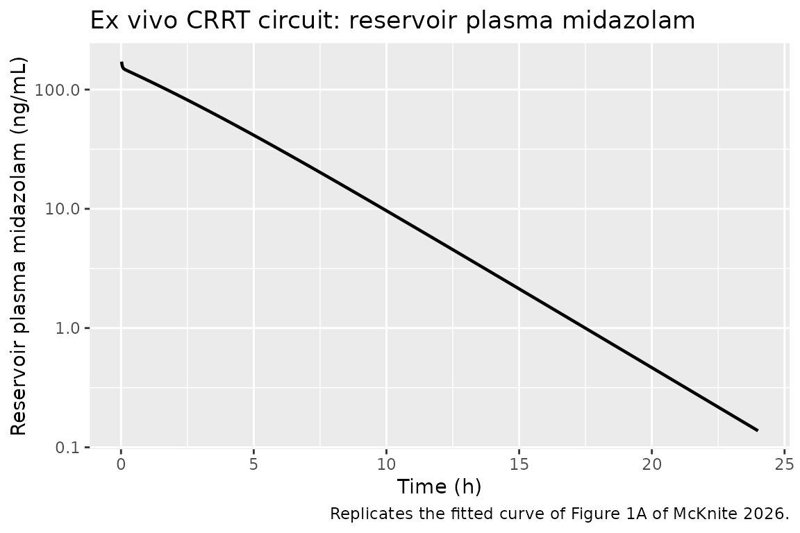
# Where the drug goes. Replicates the compartmental picture of Figure 1B.
sim_exvivo |>
  dplyr::filter(arm == "Ex vivo") |>
  dplyr::select(time, dplyr::all_of(states)) |>
  tidyr::pivot_longer(-time, names_to = "state", values_to = "amount") |>
  ggplot(aes(time, amount * 1000, colour = state)) +
  geom_line(linewidth = 0.7) +
  labs(x = "Time (h)", y = "Midazolam (ug)", colour = NULL,
       title = "Ex vivo circuit: amount by compartment",
       caption = "Compartments as drawn in Figure 1B of McKnite 2026.")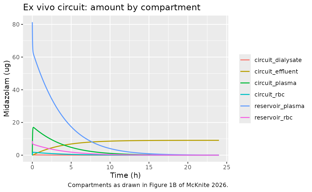
Bridge to the paper’s dosing conclusion (Figure 6)
The paper’s dosing recommendation is 0.04 mg/kg/h for neonates and 0.1 mg/kg/h for every older group, both inside the standard ranges (0.015-0.06 and 0.05-0.12 mg/kg/h respectively), which is why it concludes that “no dosing adjustment for midazolam is needed in children supported with CRRT” (Discussion). Results 3.6 gives the whole-body midazolam clearance of its virtual critically ill populations as 3.6-11.3 mL/min/kg. Placing the circuit clearance from the table above against that range shows the circuit as a minor but age-dependent contributor.
bridge <- cmp_cl |>
  dplyr::left_join(arms |> dplyr::select(arm, wt_kg), by = "arm") |>
  dplyr::filter(!is.na(wt_kg)) |>
  dplyr::mutate(
    cl_mlmin = cl_closed * 1000 / 60,
    cl_mlminkg = cl_mlmin / wt_kg,
    pct_of_low_body_cl = 100 * cl_mlminkg / 3.6,
    pct_of_high_body_cl = 100 * cl_mlminkg / 11.3
  )

# The circuit is a device: its absolute clearance is set by the membrane and
# the adsorptive surface, not by the patient, so it must be nearly flat in
# mL/min across a 16-fold weight range. Realised 2.91-3.74 mL/min.
stopifnot(diff(range(bridge$cl_mlmin)) < 1.5)
# Per kilogram it must therefore fall monotonically with weight.
stopifnot(all(diff(bridge$cl_mlminkg) < 0))
# And it must stay below even the lowest whole-body clearance the paper
# reports, so the circuit can never be the dominant elimination route.
stopifnot(all(bridge$cl_mlminkg < 3.6))

knitr::kable(
  bridge |>
    dplyr::select(arm, wt_kg, cl_mlmin, cl_mlminkg,
                  pct_of_low_body_cl, pct_of_high_body_cl) |>
    dplyr::rename(
      "Age group" = arm, "Weight (kg)" = wt_kg,
      "Circuit CL (mL/min)" = cl_mlmin,
      "Circuit CL (mL/min/kg)" = cl_mlminkg,
      "% of 3.6 mL/min/kg" = pct_of_low_body_cl,
      "% of 11.3 mL/min/kg" = pct_of_high_body_cl
    ),
  digits = 3,
  caption = "Circuit clearance against the whole-body midazolam clearance range of 3.6-11.3 mL/min/kg reported in Results 3.6."
)| Age group | Weight (kg) | Circuit CL (mL/min) | Circuit CL (mL/min/kg) | % of 3.6 mL/min/kg | % of 11.3 mL/min/kg |
|---|---|---|---|---|---|
| Neonatal | 3.5 | 2.911 | 0.832 | 23.107 | 7.361 |
| Infant | 5.1 | 2.967 | 0.582 | 16.161 | 5.149 |
| Child | 14.0 | 3.290 | 0.235 | 6.528 | 2.080 |
| School age | 29.7 | 3.533 | 0.119 | 3.304 | 1.053 |
| Adolescent | 56.6 | 3.739 | 0.066 | 1.835 | 0.585 |
The gradient is the interesting part. Because the circuit’s adsorptive surface and membrane are device properties, the circuit removes roughly the same 2.9-3.7 mL/min whatever the patient’s size, so per kilogram it falls from 0.83 mL/min/kg in a 3.5 kg neonate to 0.066 mL/min/kg in a 56.6 kg adolescent – a 13-fold difference. That is consistent with the shape of the paper’s own recommendation: the neonatal model-informed dose of 0.04 mg/kg/h sits near the top of the standard neonatal range of 0.015-0.06, whereas 0.1 mg/kg/h sits mid-range for every older group. The module was not fitted to the dosing figure, so this is an independent consistency check rather than a reconstruction of it.
Assumptions and deviations
Errata and source problems
-
The ex vivo dialysate flow unit is wrong as
printed. Methods 2.5 gives the ex vivo prescription as
“blood flow rate, 80 mL/min; dialysate flow rate, 400 mL/min;
pre-blood pump, 300 mL/h; replacement fluids, 100 mL/h; and patient
fluid removal, 0 mL/h.” Every other flow in that sentence is mL/h.
Read as printed, 400 mL/min is 24 L/h, which exceeds the PrisMax
platform’s maximum dialysate rate and would put dialysate flow at five
times blood flow; the deposited MoBi project stores the patient
dialysate flow at mL/h scale (0.003483 L/min = 209 mL/h).
qdiais therefore set to 400 mL/h. -
The HF1000 membrane surface area disagrees between the
Methods and Table S3. Methods 2.5 says 1.2 m^2 for the ex vivo
build; Table S3 lists 1.1 m^2 for the HF1000. The Methods value is used,
because it is what the ex vivo circuit was parameterised with. The
choice is numerically immaterial:
D * SA / his around 1.4e5 L/h either way, five orders of magnitude above every other circuit flow, so the dialysate is at quasi-equilibrium under both readings (see the dialysate gate above). -
The reported
V_maxunit is not dimensionally consistent with the rate law it parameterises. Results 3.3 prints “V max of 0.002 L/min”, but the rate law isV_max * C / (C + K_m), in whichC / (C + K_m)is dimensionless, soV_maxmust carry amount per time. The deposited project is itself inconsistent: the parameter is declared with dimension “Inversed time” and display unit 1/min, while the formula that consumes it declares its argument as “Concentration (molar) per time”. The numeric value is unambiguous (0.00245 in the Open Systems Pharmacology base units), so it is carried here as an amount-per-time in the role the rate law requires, converted to 0.047888 mg/h.K_mhas no such problem: 1.1 umol/L in the project reproduces the printed 1100 pmol/mL exactly. -
V_maxis taken unrounded from the deposited project, not from the printed value. Results 3.3 prints 0.002 at one significant figure; the project’s optimized reaction block stores 0.00245, tagged as updated by “Parameter Identification 2” on 2022-08-15. The executable artifact is taken as authoritative over the rounded print. -
UFRin Tables S2 and S4 is mapped to the patient fluid removal rate. Those tables label the column “Ultrafiltration rate” while Methods 2.5 uses the PrisMax term “patient fluid removal”. The two coincide if the tabulated number is the net rate, which is the platform’s own convention, but the paper does not state it. If it were instead the gross filtrate flow it would map toQ_FILrather thanQ_PFR, which would change the effluent flow by at most a few tenths of a litre per hour and the circuit clearance by under 1%, because the filter contributes only a small fraction of total circuit removal.
Parameters not printed in the paper
Four values are taken from the authors’ deposited MoBi 10.0 project,
supplied as part of Appendix S1. It is a SQLite database and the values
below were read from it directly; none of them appears in the paper’s
text, tables or supplement. Values are recorded in Open Systems
Pharmacology base units, which frequently disagree with the
stored displayUnit, so each was converted from the base
unit rather than from what the project displays.
-
dfilter = 0.594 dm^2/h(0.99 cm^2/min). The HF1000 container’sMembraneDiffusionCoefficient, stored as 0.0099 in the dm^2/min base unit. Methods 2.5 says the coefficient was optimized alongside the elimination rate constant but never reports it. -
krbc = 0.2492, the red-cell to plasma concentration ratio. PK-Sim computes this internally rather than exposing it as an input, so it was evaluated from the project’s own stored formulaK_rbc = (f_water_rbc + f_lipids_rbc * 10^LogMA + f_proteins_rbc * KProt) * fuwithKProt = (0.81 + 0.11 * 10^LogMA) / 24.92 * 5,LogMA = Lipophilicity = 2.98577(Table 1 rounds this to 2.99),f_water_rbc = 0.625,f_lipids_rbc = 0.005,f_proteins_rbc = 0.325andfu = 0.02, every one of which is stored in the project. The derivation checks out independently: the implied blood-to-plasma ratiokrbc * hct + 1 - hctis 0.775 at hematocrit 0.30, which is the accepted value for midazolam. No literature blood-to-plasma ratio was substituted. -
permrbc = 0.3004 dm/h, the plasma to red-cell membrane permeability, from the project’s stored formulaP = (MWEff * 1e9 / 336)^-6 * 10^LogMA / 5 * 1e-5with the Table 1 effective molecular weight of 286.78 g/mol. -
satovrbc = 1.002e6 1/dm, the red-cell exchange area per unit red-cell volume: the project’sSurface/Volume ratio (blood cells)of 167000 1/cm multiplied by the Open Systems Pharmacology accessibility factor of 0.6 that appears in its exchange-area formula.
The last three enter only the plasma / red-cell exchange, whose
permeability-surface product comes out two to three orders of magnitude
larger than the blood flow. The two phases therefore remain at
equilibrium throughout (verified above to within 0.1%), so the model’s
behaviour depends on krbc but is insensitive to
permrbc and satovrbc. They are carried
explicitly rather than replaced by an instantaneous-equilibrium
assumption so that the assumption stays visible and testable.
Structural simplifications
-
The whole-body models are not reproduced. Only the
circuit module is; see the scope table at the top. A user who wants
circuit-plus-body behaviour should attach these
circuit_*states to a body model’s venous blood compartment in place of thereservoir_*pair, which is exactly what the authors did. -
No adsorption sink in the effluent state. The
deposited project’s
MidazolamDegradationreaction is scoped to every container taggedPrisMaxthat is not taggedDialysate, which instantiates it in the filter plasma, the filter red cells and the terminal dialysate bag. The bag is downstream of everything and cannot influence any upstream concentration, so the third instance is an artifact of the container tagging rather than a mechanism;circuit_effluentis therefore a pure accumulation state. This affects the reported cumulative effluent amount but no concentration. -
Equation 3 is not carried.
Q_PR, the total fluid removal rate, appears in no mass transfer in either the printed equations or the deposited project. - Per-filter dialysate volumes are scaled, not sourced. Table S3 tabulates membrane surface area, wall thickness, filter blood volume and circuit blood volume for all eight filters but no dialysate-side volume; Methods 2.5 gives it only for the HF1000. The five clinical arms scale it with membrane surface area from that anchor. The dialysate gate above shows a ten-fold change in this volume moves the observed concentration by under 1%.
- Hematocrit is held at 0.30 in every arm. That is the ex vivo value (Methods 2.5). Methods 2.9 states that critical illness reduced hematocrit by 28% relative to healthy age-matched children but does not print the healthy reference values, so no per-age-group hematocrit is recoverable; 0.30 is in any case a reasonable critically ill pediatric value and applying it uniformly keeps the comparison across arms clean.
-
The reservoir is retained in the clinical arms as a
numerical device. The quantity read off those arms is
Dose / AUCinf, which is independent of reservoir volume; no time-course prediction is read from them.
Unreported variability
The circuit module carries no between-subject variability and no
residual error, and this is faithful rather than a simplification: the
two Michaelis-Menten constants were obtained by Monte Carlo parameter
identification in PK-Sim against ex vivo concentration data (Methods
2.5), and no residual-error model, standard deviation, confidence
interval or between-replicate variance is reported anywhere in the
paper, the supplement or the deposited project. propSd is
held at fixed(0) rather than invented. A user who wants a
stochastic circuit must supply their own error model.