Basimglurant PK and exposure-dizziness (Cosson 2018)
Source:vignettes/articles/Cosson_2018_basimglurant_exposure_dizziness.Rmd
Cosson_2018_basimglurant_exposure_dizziness.RmdModel and source
Cosson 2018 reports two models fitted in sequence: a population PK
model of oral modified-release (MR) basimglurant fitted in NONMEM, and a
logistic regression of dizziness incidence on the individual predicted
Day-1 peak concentration (Cmax,Day1) fitted with glm() in
R. They are packaged as two model files:
-
Cosson_2018_basimglurant– population PK. -
Cosson_2018_basimglurant_dizziness– exposure-dizziness logistic model, whose exposure columnCMAXis simulated with the PK model.
pk_mod <- readModelDb("Cosson_2018_basimglurant")
dz_mod <- readModelDb("Cosson_2018_basimglurant_dizziness")
pk_ui <- rxode2::rxode(pk_mod)
#> ℹ parameter labels from comments will be replaced by 'label()'
dz_ui <- rxode2::rxode(dz_mod)- Citation: Cosson V, Schaedeli-Stark F, Arab-Alameddine M, Chavanne C, Guerini E, Derks M, Jaeschke G, Lindemann L, Umbricht D, Santarelli L. Population Pharmacokinetic and Exposure-dizziness Modeling for a Metabotropic Glutamate Receptor Subtype 5 Negative Allosteric Modulator in Major Depressive Disorder Patients. Clin Transl Sci. 2018;11(5):523-531. doi:10.1111/cts.12566.
- PK description: Two-compartment population PK model for oral modified-release basimglurant (RO4917523, an mGlu5 negative allosteric modulator) in healthy adults and adults with major depressive disorder (Cosson 2018, 288 participants pooled from four phase I trials and one phase II trial). Absorption is a chain of three first-order transit compartments (depot plus two transit compartments, all at rate Ktr) after a lag time, with separate Ktr and lag-time estimates in the fed and fasted states; elimination is first order. Covariates: Asian race on fasted Ktr and on relative bioavailability, smoking and male sex on CL/F, body weight and smoking on Vc/F, male sex on Q/F, and body weight and male sex on Vp/F. The typical subject is a non-Asian female non-smoker weighing 71 kg. The companion Cmax-driven dizziness model is Cosson_2018_basimglurant_dizziness.
- Dizziness description: Logistic-regression exposure-safety model for the probability of dizziness (first occurrence, any severity) in adults with major depressive disorder taking oral modified-release basimglurant (Cosson 2018, 310 phase II patients: placebo, 0.5 mg or 1.5 mg once daily). The linear predictor is -2.970 + 0.412 * Cmax,Day1, where Cmax,Day1 (ng/mL) is the individual predicted peak concentration over the first 24-hour dosing interval, set to 0 for placebo patients. No PK layer and no ODE: exposure enters as the static per-patient column CMAX, simulated with modellib(‘Cosson_2018_basimglurant’). No between-subject random effect and no residual error are estimated (Bernoulli likelihood, R glm).
- Article: https://doi.org/10.1111/cts.12566 (open access, PMC6132363)
Population
The PK analysis pooled 3,533 plasma concentrations from 288 participants in five trials: 88 healthy adults in four phase I studies (an MR-vs-IR formulation and food-effect crossover, two drug-interaction studies with fluvoxamine and carbamazepine, and a single- and multiple-dose study in Japanese and Caucasian volunteers) and 200 adults with major depressive disorder (MDD) in the phase II adjunctive-therapy trial NCT01437657. Basimglurant MR was given orally once daily at 0.2 to 1.5 mg. 273 participants took it with food, 35 fasted, and 20 under both conditions; 58% were female and 17% Asian, with a median weight of 71.9 kg and a median age of 43.5 years (Cosson 2018 Methods and Results “PK results”; the paper has no demographics table).
The exposure-dizziness analysis used 310 phase II patients: 110 on placebo (6 with dizziness), 99 on 0.5 mg (3) and 101 on 1.5 mg (26). Only the first occurrence of dizziness, of any severity, was analysed.
str(pk_ui$population)
#> List of 13
#>  $ species       : chr "human"
#>  $ n_subjects    : int 288
#>  $ n_studies     : int 5
#>  $ n_observations: int 3533
#>  $ age_median    : chr "43.5 years"
#>  $ weight_median : chr "71.9 kg"
#>  $ sex_female_pct: num 58
#>  $ race_ethnicity: Named num 17
#>   ..- attr(*, "names")= chr "Asian"
#>  $ disease_state : chr "88 healthy adults (four phase I trials, including healthy Japanese and Caucasian participants) and 200 adults w"| __truncated__
#>  $ dose_range    : chr "0.2, 0.5, 0.7, 1 or 1.5 mg basimglurant modified-release tablet orally once daily, single and multiple doses"
#>  $ regions       : chr "Phase I sites in France and the United States; phase II sites not stated"
#>  $ co_medication : chr "Two phase I trials co-administered fluvoxamine or carbamazepine (drug-interaction studies); phase II patients c"| __truncated__
#>  $ notes         : chr "Cosson 2018 Methods 'Patient population and study design' and Results 'PK results'. 273 participants received b"| __truncated__
str(dz_ui$population)
#> List of 7
#>  $ species       : chr "human"
#>  $ n_subjects    : int 310
#>  $ n_studies     : int 1
#>  $ n_observations: chr "310 binary first-occurrence dizziness records (one per patient; landmark analysis)"
#>  $ disease_state : chr "adults with major depressive disorder and inadequate response to ongoing antidepressant treatment (adjunctive b"| __truncated__
#>  $ dose_range    : chr "placebo (n = 110), 0.5 mg (n = 99) or 1.5 mg (n = 101) basimglurant modified-release once daily"
#>  $ notes         : chr "Cosson 2018 Results 'Exposure-safety results'. Dizziness was reported by 6/110 placebo, 3/99 (0.5 mg) and 26/10"| __truncated__
Source trace
Every ini() value carries an in-file comment naming its
source. The table collects them.
| Parameter | Value | Source location |
|---|---|---|
lcl |
log(8.87) L/h | Table 1, CL; CL/F equation |
lvc |
log(231) L | Table 1, Vc; Vc/F equation |
lq |
log(31.0) L/h | Table 1, Q; Q/F equation |
lvp |
log(1140) L | Table 1, Vp; Vp/F equation |
lktr_fasted |
log(4.52) 1/h | Table 1, Ktr fasted; Ktr equation |
lktr_fed |
log(0.999) 1/h | Table 1, Ktr fed; Ktr equation |
ltlag_fasted |
log(0.212) h | Table 1, lag time fasted; Tlag equation |
ltlag_fed |
log(0.120) h | Table 1, lag time fed; Tlag equation |
e_race_asian_ktr_fasted |
-0.588 | Table 1 (magnitude 0.588); sign from Ktr equation
(1 - 0.588 * ETHN)
|
e_sex_cl |
0.401 | Table 1, gender on CL; CL/F equation |
e_smoke_cl |
1.08 | Table 1, smoking on CL; CL/F equation |
e_wt_vc |
0.879 | Table 1, body weight on Vc; Vc/F equation
(WT/71)^0.879
|
e_smoke_vc |
0.397 | Table 1, smoking on Vc; Vc/F equation |
e_sex_q |
-0.213 | Table 1, gender on Q; Q/F equation |
e_wt_vp |
1.71 | Table 1, body weight on Vp; Vp/F equation
(WT/71)^1.71
|
e_sex_vp |
-0.434 | Table 1, gender on Vp; Vp/F equation |
e_race_asian_fdepot |
1.26 (ratio) | Table 1, ethnicity on F; Figure 2; Discussion (see Errata 1) |
etalcl, etalvc, etalq,
etalvp block |
CV 71.3, 25.9, 36.3, 37.4%; six correlations | Table 1, BSV and correlation rows |
etalktr_fasted |
CV 41.9% | Table 1 |
etalktr_fed |
CV 53.8% | Table 1 |
propSd |
0.262 | Table 1, proportional residual error (see Errata 2) |
logit_ref |
-2.970 | Table 2, intercept |
e_cmax_logit |
0.412 per ng/mL | Table 2, slope |
addSd_prob_dizziness |
0.001 (fixed) | not from the source; placeholder for the Bernoulli likelihood |
| Absorption chain | depot + 2 transit compartments, all at Ktr | Results: “a chain of three compartments, including the depot compartment” |
| Disposition | 2 compartments, first-order elimination | Abstract; Results “PK results” |
| Dizziness link | logit(p) = -2.970 + 0.412 * Cmax,Day1 |
Methods “Exposure-safety analysis”; Table 2 |
The covariate equations printed in Results “PK results” are, with the typical subject a non-Asian, non-smoking 71 kg female (Figure 2 caption):
Ktr  = 4.52 * (1 - FOOD) * (1 - 0.588 * ETHN) + 0.999 * FOOD
Tlag = 0.212 * (1 - FOOD) + 0.12 * FOOD
CL/F = 8.87 * (1 + 1.08 * SMOK) * (1 + 0.401 * SEX)
Vc/F = 231 * (WT / 71)^0.879 * (1 + 0.397 * SMOK)
Q/F  = 31.0 * (1 - 0.213 * SEX)
Vp/F = 1140 * (1 - 0.434 * SEX) * (WT / 71)^1.71
F    = 1 + 1.26 * ETHN        (printed; encoded as 1.26^ETHN, Errata 1)
SEX is a male indicator in the paper; the model stores
the canonical SEXF (1 = female) and applies each sex effect
to 1 - SEXF. FOOD becomes FED,
SMOK becomes SMOKE, and ETHN
becomes RACE_ASIAN. Between-subject variances are
omega^2 = log(CV^2 + 1) from the Table 1 %CVs.
Typical-value checks against the paper’s derived quantities
These checks use the typical-value model (zeroRe()), so
both sides are deterministic and the tolerances are tight.
pk_typ <- rxode2::zeroRe(pk_mod)
#> ℹ parameter labels from comments will be replaced by 'label()'

ref_cov <- data.frame(SEXF = 1, SMOKE = 0, RACE_ASIAN = 0, WT = 71, FED = 1)

# Typical apparent parameters for one covariate combination.
typ_par <- function(...) {
  cv <- ref_cov
  ov <- list(...)
  for (nm in names(ov)) cv[[nm]] <- ov[[nm]]
  ev <- data.frame(id = 1L, time = 0, amt = 0, evid = 0L, cmt = "central")
  o <- as.data.frame(rxode2::rxSolve(pk_typ, events = cbind(ev, cv)))
  c(cl = o$cl[1], vc = o$vc[1], q = o$q[1], vp = o$vp[1], f = o$fdepot[1])
}

# Terminal half-life of a two-compartment system from its apparent parameters.
thalf_term <- function(p) {
  k <- p[["cl"]] / p[["vc"]]
  k12 <- p[["q"]] / p[["vc"]]
  k21 <- p[["q"]] / p[["vp"]]
  s <- k + k12 + k21
  beta <- (s - sqrt(s^2 - 4 * k * k21)) / 2
  log(2) / beta
}

p_female <- typ_par()
#> ℹ omega/sigma items treated as zero: 'etalcl', 'etalvc', 'etalq', 'etalvp', 'etalktr_fasted', 'etalktr_fed'
p_male <- typ_par(SEXF = 0)
#> ℹ omega/sigma items treated as zero: 'etalcl', 'etalvc', 'etalq', 'etalvp', 'etalktr_fasted', 'etalktr_fed'
p_smoker <- typ_par(SMOKE = 1)
#> ℹ omega/sigma items treated as zero: 'etalcl', 'etalvc', 'etalq', 'etalvp', 'etalktr_fasted', 'etalktr_fed'
Cosson 2018 Discussion quotes terminal half-lives of 129 h (typical
female), 63 h (typical male) and 76 h (typical smoker), and “effective”
half-lives of 107 h (female) and 49 h (male). The effective values are
reproduced by log(2) * Vss / CL, i.e. log(2)
times the mean residence time.
thalf_tab <- tibble::tribble(
  ~quantity, ~published,
  "Terminal t1/2, typical female (h)", 129,
  "Terminal t1/2, typical male (h)", 63,
  "Terminal t1/2, typical smoker (h)", 76,
  "Effective t1/2 = ln2*Vss/CL, female (h)", 107,
  "Effective t1/2 = ln2*Vss/CL, male (h)", 49
) |>
  mutate(
    model = c(
      thalf_term(p_female), thalf_term(p_male), thalf_term(p_smoker),
      log(2) * (p_female[["vc"]] + p_female[["vp"]]) / p_female[["cl"]],
      log(2) * (p_male[["vc"]] + p_male[["vp"]]) / p_male[["cl"]]
    ),
    pct_diff = 100 * (model - published) / published
  )
knitr::kable(thalf_tab, digits = 2, caption = "Half-lives quoted in the Cosson 2018 Discussion.")| quantity | published | model | pct_diff |
|---|---|---|---|
| Terminal t1/2, typical female (h) | 129 | 129.06 | 0.05 |
| Terminal t1/2, typical male (h) | 63 | 63.49 | 0.77 |
| Terminal t1/2, typical smoker (h) | 76 | 76.40 | 0.52 |
| Effective t1/2 = ln2*Vss/CL, female (h) | 107 | 107.14 | 0.13 |
| Effective t1/2 = ln2*Vss/CL, male (h) | 49 | 48.88 | -0.26 |
# Published values are rounded to whole hours, so 1.5% covers the rounding.
stopifnot(all(abs(thalf_tab$pct_diff) < 1.5))
Figure 2 – covariate effects on the apparent disposition parameters
Figure 2 shows each covariate effect as a percent change from the typical subject. Low and high weight are 52 and 100 kg.
fig2 <- bind_rows(
  tibble(level = "Smoker", p = list(typ_par(SMOKE = 1))),
  tibble(level = "Male", p = list(typ_par(SEXF = 0))),
  tibble(level = "Asian", p = list(typ_par(RACE_ASIAN = 1))),
  tibble(level = "Low weight (52 kg)", p = list(typ_par(WT = 52))),
  tibble(level = "High weight (100 kg)", p = list(typ_par(WT = 100)))
) |>
  mutate(
    `CL/F` = sapply(p, function(x) x[["cl"]] / x[["f"]]),
    `Vc/F` = sapply(p, function(x) x[["vc"]] / x[["f"]]),
    `Q/F` = sapply(p, function(x) x[["q"]] / x[["f"]]),
    `Vp/F` = sapply(p, function(x) x[["vp"]] / x[["f"]])
  ) |>
  select(-p) |>
  pivot_longer(-level, names_to = "parameter", values_to = "value") |>
  mutate(
    ref = case_when(
      parameter == "CL/F" ~ p_female[["cl"]],
      parameter == "Vc/F" ~ p_female[["vc"]],
      parameter == "Q/F" ~ p_female[["q"]],
      parameter == "Vp/F" ~ p_female[["vp"]]
    ),
    pct_change = 100 * (value / ref - 1)
  )
#> ℹ omega/sigma items treated as zero: 'etalcl', 'etalvc', 'etalq', 'etalvp', 'etalktr_fasted', 'etalktr_fed'
#> ℹ omega/sigma items treated as zero: 'etalcl', 'etalvc', 'etalq', 'etalvp', 'etalktr_fasted', 'etalktr_fed'
#> ℹ omega/sigma items treated as zero: 'etalcl', 'etalvc', 'etalq', 'etalvp', 'etalktr_fasted', 'etalktr_fed'
#> ℹ omega/sigma items treated as zero: 'etalcl', 'etalvc', 'etalq', 'etalvp', 'etalktr_fasted', 'etalktr_fed'
#> ℹ omega/sigma items treated as zero: 'etalcl', 'etalvc', 'etalq', 'etalvp', 'etalktr_fasted', 'etalktr_fed'

ggplot(fig2, aes(pct_change, level)) +
  geom_vline(xintercept = 0) +
  geom_vline(xintercept = c(-20, 20), linetype = "dashed") +
  geom_point(shape = 15, colour = "navy", size = 2.5) +
  facet_wrap(~parameter) +
  labs(
    x = "Change from typical subject (%)", y = NULL,
    caption = "Replicates Figure 2 of Cosson 2018 (typical subject: female, non-Asian, non-smoker, 71 kg)."
  )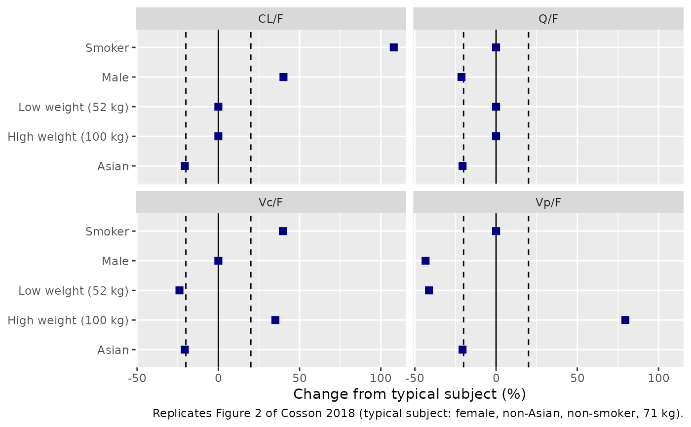
fig2 |>
  select(level, parameter, pct_change) |>
  pivot_wider(names_from = parameter, values_from = pct_change) |>
knitr::kable(digits = 1, caption = "Percent change from the typical subject in the apparent parameters.")| level | CL/F | Vc/F | Q/F | Vp/F |
|---|---|---|---|---|
| Smoker | 108.0 | 39.7 | 0.0 | 0.0 |
| Male | 40.1 | 0.0 | -21.3 | -43.4 |
| Asian | -20.6 | -20.6 | -20.6 | -20.6 |
| Low weight (52 kg) | 0.0 | -23.9 | 0.0 | -41.3 |
| High weight (100 kg) | 0.0 | 35.1 | 0.0 | 79.6 |
The model reproduces every symbol in Figure 2 – smoker +108% on CL/F, male +40% on CL/F, -21% on Q/F and -43% on Vp/F, weight -24%/+35% on Vc/F and -41%/+80% on Vp/F, and Asian -21% on all four apparent parameters (the reciprocal of the 1.26 relative bioavailability) – with one exception. The Vc/F panel of Figure 2 has a symbol labelled “Male” at +40% and none for smoking, but the model has no sex effect on Vc/F; +39.7% is the smoking effect, and the Vc/F row “Smoker” above shows it. The label in the figure is treated as a mislabel (Errata 3).
Steady-state exposure claims in the Discussion
ss_profile <- function(cov, dose = 1.5) {
  ev <- rxode2::et(amt = dose, cmt = "depot", ii = 24, addl = 59) |>
    rxode2::et(seq(1416, 1440, by = 0.05), cmt = "central") |>
    as.data.frame()
  ev$id <- 1L
  as.data.frame(rxode2::rxSolve(
    pk_typ,
    events = cbind(ev, cov), maxsteps = 1e6
  ))
}
auc_trap <- function(t, c) sum(diff(t) * (head(c, -1) + tail(c, -1)) / 2)
ss_metric <- function(cov) {
  o <- ss_profile(cov)
  c(auc = auc_trap(o$time, o$Cc), cmax = max(o$Cc))
}
m_f <- ss_metric(ref_cov)
#> ℹ omega/sigma items treated as zero: 'etalcl', 'etalvc', 'etalq', 'etalvp', 'etalktr_fasted', 'etalktr_fed'
m_m <- ss_metric(transform(ref_cov, SEXF = 0))
#> ℹ omega/sigma items treated as zero: 'etalcl', 'etalvc', 'etalq', 'etalvp', 'etalktr_fasted', 'etalktr_fed'
m_s <- ss_metric(transform(ref_cov, SMOKE = 1))
#> ℹ omega/sigma items treated as zero: 'etalcl', 'etalvc', 'etalq', 'etalvp', 'etalktr_fasted', 'etalktr_fed'

ss_tab <- tibble::tribble(
  ~claim, ~published_pct,
  "Male vs female, AUC,ss", -30,
  "Male vs female, Cmax,ss", -20,
  "Smoker vs non-smoker, AUC,ss", -52
) |>
  mutate(model_pct = c(
    100 * (m_m[["auc"]] / m_f[["auc"]] - 1),
    100 * (m_m[["cmax"]] / m_f[["cmax"]] - 1),
    100 * (m_s[["auc"]] / m_f[["auc"]] - 1)
  ))
knitr::kable(ss_tab, digits = 1, caption = "Steady-state exposure differences quoted in the Cosson 2018 Discussion (1.5 mg fed).")| claim | published_pct | model_pct |
|---|---|---|
| Male vs female, AUC,ss | -30 | -28.6 |
| Male vs female, Cmax,ss | -20 | -21.7 |
| Smoker vs non-smoker, AUC,ss | -52 | -51.9 |
Food and ethnicity effects on Day-1 absorption
The Discussion states that food reduced Day-1 Cmax by about 30% and delayed Tmax by 2.5 h relative to the fasted state, and that ethnicity delayed absorption by 1.5 h in Asian subjects under fasted conditions only.
day1 <- function(cov, dose = 0.5) {
  ev <- rxode2::et(amt = dose, cmt = "depot") |>
    rxode2::et(seq(0, 24, by = 0.01), cmt = "central") |>
    as.data.frame()
  ev$id <- 1L
  o <- as.data.frame(rxode2::rxSolve(pk_typ, events = cbind(ev, cov)))
  c(cmax = max(o$Cc), tmax = o$time[which.max(o$Cc)])
}
d_fed <- day1(ref_cov)
#> ℹ omega/sigma items treated as zero: 'etalcl', 'etalvc', 'etalq', 'etalvp', 'etalktr_fasted', 'etalktr_fed'
d_fast <- day1(transform(ref_cov, FED = 0))
#> ℹ omega/sigma items treated as zero: 'etalcl', 'etalvc', 'etalq', 'etalvp', 'etalktr_fasted', 'etalktr_fed'
d_fast_asian <- day1(transform(ref_cov, FED = 0, RACE_ASIAN = 1))
#> ℹ omega/sigma items treated as zero: 'etalcl', 'etalvc', 'etalq', 'etalvp', 'etalktr_fasted', 'etalktr_fed'
d_fed_asian <- day1(transform(ref_cov, FED = 1, RACE_ASIAN = 1))
#> ℹ omega/sigma items treated as zero: 'etalcl', 'etalvc', 'etalq', 'etalvp', 'etalktr_fasted', 'etalktr_fed'

abs_tab <- tibble::tribble(
  ~claim, ~published, ~model,
  "Fed vs fasted, Day-1 Cmax change (%)", -30, 100 * (d_fed[["cmax"]] / d_fast[["cmax"]] - 1),
  "Fed vs fasted, Tmax delay (h)", 2.5, d_fed[["tmax"]] - d_fast[["tmax"]],
  "Asian vs non-Asian fasted, Tmax delay (h)", 1.5, d_fast_asian[["tmax"]] - d_fast[["tmax"]],
  "Asian vs non-Asian fed, Tmax delay (h)", 0, d_fed_asian[["tmax"]] - d_fed[["tmax"]]
)
knitr::kable(abs_tab, digits = 2, caption = "Day-1 absorption claims in the Cosson 2018 Discussion (typical female, 71 kg).")| claim | published | model |
|---|---|---|
| Fed vs fasted, Day-1 Cmax change (%) | -30.0 | -29.01 |
| Fed vs fasted, Tmax delay (h) | 2.5 | 3.23 |
| Asian vs non-Asian fasted, Tmax delay (h) | 1.5 | 1.49 |
| Asian vs non-Asian fed, Tmax delay (h) | 0.0 | 0.00 |
stopifnot(
  abs(abs_tab$model[1] - (-30)) < 3,
  abs(abs_tab$model[3] - 1.5) < 0.1,
  abs(abs_tab$model[4]) < 0.01
)
The model’s food-related Tmax delay is about 3.2 h against the 2.5 h quoted. The Day-1 Cmax reduction and the Figure 3 steady-state profiles (next section) both match, so the quoted 2.5 h is recorded as a known deviation rather than gated; the paper does not say how that figure was derived.
Figure 3 – steady-state typical profiles by covariate
Figure 3 shows population-predicted steady-state profiles over one dosing interval for each combination of smoking, sex, ethnicity and weight (52, 71, 100 kg). The dose is not stated in the caption; 1.5 mg once daily with food reproduces every non-Asian curve. The trough (t = 0) and peak values below were read from the vector paths of the published figure (precision about 0.01 ng/mL).
fig3_pub <- tibble::tribble(
  ~SMOKE, ~RACE_ASIAN, ~SEXF, ~WT, ~trough_pub, ~peak_pub,
  0, 0, 1, 52, 5.48, 9.83,
  0, 0, 1, 71, 5.65, 9.27,
  0, 0, 1, 100, 5.75, 8.65,
  0, 0, 0, 52, 3.36, 7.82,
  0, 0, 0, 71, 3.56, 7.26,
  0, 0, 0, 100, 3.78, 6.71,
  1, 0, 1, 52, 2.18, 5.44,
  1, 0, 1, 71, 2.32, 5.01,
  1, 0, 1, 100, 2.48, 4.60,
  1, 0, 0, 52, 1.22, 4.46,
  1, 0, 0, 71, 1.36, 4.03,
  1, 0, 0, 100, 1.52, 3.63,
  0, 1, 1, 52, 8.70, 15.61,
  0, 1, 1, 71, 8.96, 14.71,
  0, 1, 1, 100, 9.13, 13.73,
  0, 1, 0, 52, 5.33, 12.41,
  0, 1, 0, 71, 5.65, 11.52,
  0, 1, 0, 100, 6.00, 10.65,
  1, 1, 1, 52, 3.46, 8.63,
  1, 1, 1, 71, 3.68, 7.95,
  1, 1, 1, 100, 3.93, 7.30,
  1, 1, 0, 52, 1.93, 7.07,
  1, 1, 0, 71, 2.16, 6.40,
  1, 1, 0, 100, 2.40, 5.76
)
fig3_cov <- fig3_pub |>
  select(SMOKE, RACE_ASIAN, SEXF, WT) |>
  mutate(id = row_number(), FED = 1)
fig3_ev <- rxode2::et(amt = 1.5, cmt = "depot", ii = 24, addl = 59) |>
  rxode2::et(seq(1416, 1440, by = 0.25), cmt = "central") |>
  as.data.frame() |>
  select(-any_of("id")) |>
  tidyr::crossing(fig3_cov) |>
  arrange(id, time, desc(evid))
fig3_sim <- as.data.frame(rxode2::rxSolve(
  pk_typ,
  events = fig3_ev, keep = c("SMOKE", "RACE_ASIAN", "SEXF", "WT"),
  maxsteps = 1e6
)) |>
  mutate(
    tad = time - 1416,
    Smoking = ifelse(SMOKE == 1, "Smoker", "Non-smoker"),
    Ethnicity = ifelse(RACE_ASIAN == 1, "Asian", "Non-Asian"),
    Sex = ifelse(SEXF == 1, "Female", "Male"),
    Weight = factor(WT, c(52, 71, 100), c("Low (52 kg)", "Median (71 kg)", "High (100 kg)"))
  )
#> ℹ omega/sigma items treated as zero: 'etalcl', 'etalvc', 'etalq', 'etalvp', 'etalktr_fasted', 'etalktr_fed'
#> Warning: multi-subject simulation without without 'omega'

ggplot(fig3_sim, aes(tad, Cc, colour = Sex, linetype = Weight)) +
  geom_line() +
  facet_grid(factor(Ethnicity, c("Non-Asian", "Asian")) ~ Smoking) +
  scale_colour_manual(values = c(Female = "tomato", Male = "steelblue")) +
  labs(
    x = "Time after dose (h)", y = "Basimglurant Cc (ng/mL)",
    caption = "Replicates Figure 3 of Cosson 2018 (typical values, 1.5 mg once daily with food, steady state)."
  )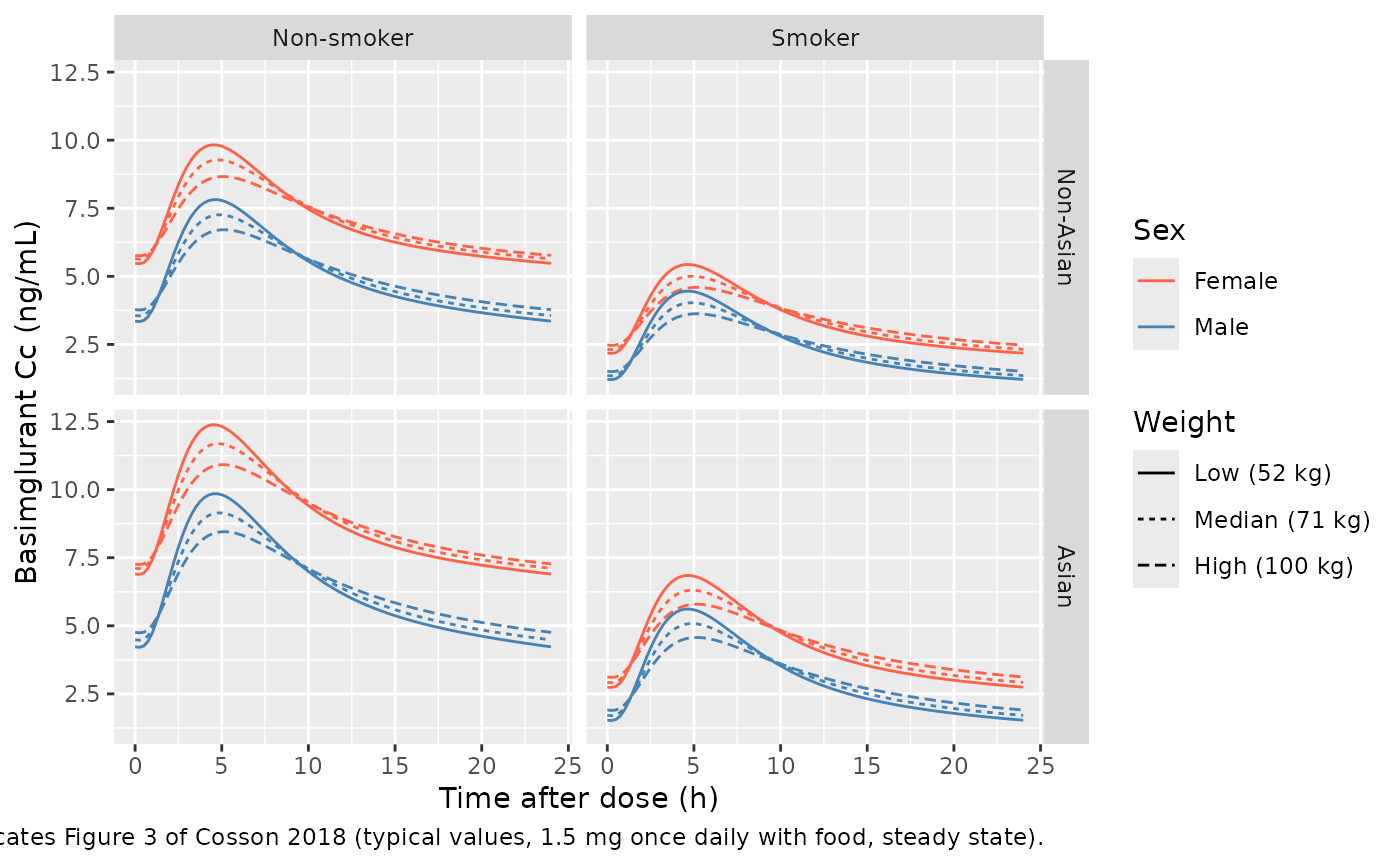
fig3_cmp <- fig3_sim |>
  group_by(SMOKE, RACE_ASIAN, SEXF, WT) |>
  summarise(trough_model = Cc[tad == 0], peak_model = max(Cc), .groups = "drop") |>
  inner_join(fig3_pub, by = c("SMOKE", "RACE_ASIAN", "SEXF", "WT")) |>
  mutate(
    trough_ratio = trough_pub / trough_model,
    peak_ratio = peak_pub / peak_model
  )
stopifnot(nrow(fig3_cmp) == 24)

fig3_cmp |>
  select(SMOKE, RACE_ASIAN, SEXF, WT, trough_pub, trough_model, peak_pub, peak_model, trough_ratio, peak_ratio) |>
knitr::kable(digits = 3, caption = "Figure 3 trough and peak: published vs model (ratio = published / model).")| SMOKE | RACE_ASIAN | SEXF | WT | trough_pub | trough_model | peak_pub | peak_model | trough_ratio | peak_ratio |
|---|---|---|---|---|---|---|---|---|---|
| 0 | 0 | 0 | 52 | 3.36 | 3.354 | 7.82 | 7.816 | 1.002 | 1.001 |
| 0 | 0 | 0 | 71 | 3.56 | 3.560 | 7.26 | 7.257 | 1.000 | 1.000 |
| 0 | 0 | 0 | 100 | 3.78 | 3.777 | 6.71 | 6.710 | 1.001 | 1.000 |
| 0 | 0 | 1 | 52 | 5.48 | 5.476 | 9.83 | 9.829 | 1.001 | 1.000 |
| 0 | 0 | 1 | 71 | 5.65 | 5.645 | 9.27 | 9.276 | 1.001 | 0.999 |
| 0 | 0 | 1 | 100 | 5.75 | 5.766 | 8.65 | 8.665 | 0.997 | 0.998 |
| 0 | 1 | 0 | 52 | 5.33 | 4.227 | 12.41 | 9.848 | 1.261 | 1.260 |
| 0 | 1 | 0 | 71 | 5.65 | 4.486 | 11.52 | 9.144 | 1.259 | 1.260 |
| 0 | 1 | 0 | 100 | 6.00 | 4.759 | 10.65 | 8.455 | 1.261 | 1.260 |
| 0 | 1 | 1 | 52 | 8.70 | 6.900 | 15.61 | 12.385 | 1.261 | 1.260 |
| 0 | 1 | 1 | 71 | 8.96 | 7.113 | 14.71 | 11.688 | 1.260 | 1.259 |
| 0 | 1 | 1 | 100 | 9.13 | 7.265 | 13.73 | 10.917 | 1.257 | 1.258 |
| 1 | 0 | 0 | 52 | 1.22 | 1.216 | 4.46 | 4.456 | 1.003 | 1.001 |
| 1 | 0 | 0 | 71 | 1.36 | 1.356 | 4.03 | 4.031 | 1.003 | 1.000 |
| 1 | 0 | 0 | 100 | 1.52 | 1.513 | 3.63 | 3.627 | 1.005 | 1.001 |
| 1 | 0 | 1 | 52 | 2.18 | 2.181 | 5.44 | 5.434 | 1.000 | 1.001 |
| 1 | 0 | 1 | 71 | 2.32 | 2.318 | 5.01 | 5.004 | 1.001 | 1.001 |
| 1 | 0 | 1 | 100 | 2.48 | 2.475 | 4.60 | 4.596 | 1.002 | 1.001 |
| 1 | 1 | 0 | 52 | 1.93 | 1.533 | 7.07 | 5.614 | 1.259 | 1.259 |
| 1 | 1 | 0 | 71 | 2.16 | 1.709 | 6.40 | 5.079 | 1.264 | 1.260 |
| 1 | 1 | 0 | 100 | 2.40 | 1.906 | 5.76 | 4.570 | 1.259 | 1.260 |
| 1 | 1 | 1 | 52 | 3.46 | 2.748 | 8.63 | 6.847 | 1.259 | 1.260 |
| 1 | 1 | 1 | 71 | 3.68 | 2.921 | 7.95 | 6.306 | 1.260 | 1.261 |
| 1 | 1 | 1 | 100 | 3.93 | 3.119 | 7.30 | 5.791 | 1.260 | 1.261 |
non_asian <- fig3_cmp |> filter(RACE_ASIAN == 0)
asian <- fig3_cmp |> filter(RACE_ASIAN == 1)
# Non-Asian curves: digitisation precision ~0.01 ng/mL on values >= 1.2 ng/mL;
# realised maximum deviation 0.7%.
stopifnot(max(abs(c(non_asian$trough_ratio, non_asian$peak_ratio) - 1)) < 0.015)
# Asian curves sit a further factor of 1.26 above the model -- the published
# figure carries 1.26^2 = 1.588 relative to non-Asian (Errata 1).
stopifnot(abs(median(c(asian$trough_ratio, asian$peak_ratio)) - 1.26) < 0.015)
All twelve non-Asian curves match within 1%. Every Asian curve in the published figure is 1.26 times the model’s Asian curve, so Figure 3 carries the Asian bioavailability factor twice (1.26^2 = 1.588 relative to the non-Asian curves). See Errata 1.
Virtual phase II cohort
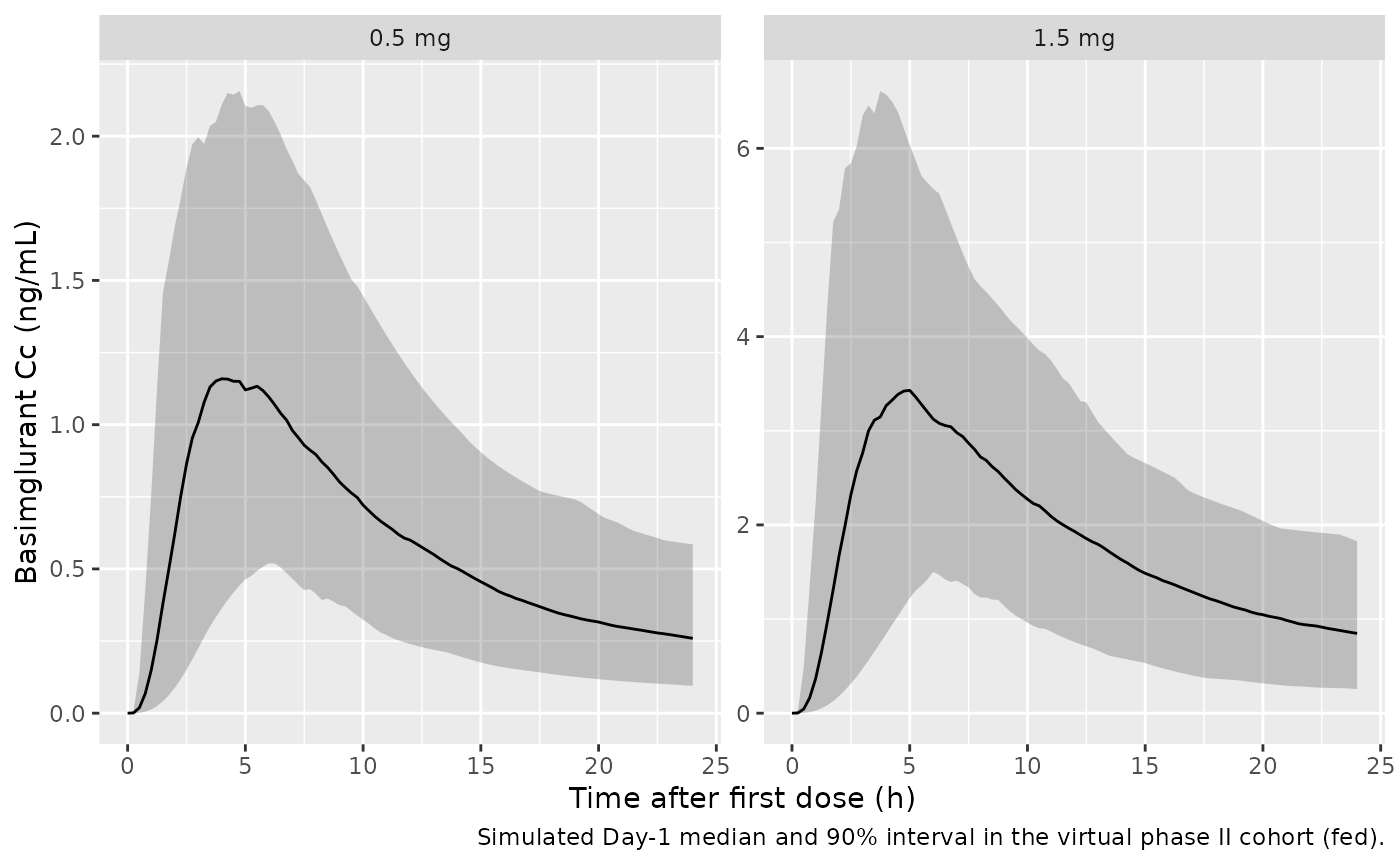
The paper reports simulated Cmax,Day1 for the phase II MDD population (Table 3) and the individual predicted values of the analysed patients (Results “Exposure-safety results”). The phase II covariate distribution is not published; the cohort below uses the overall analysis-population values (58% female, 17% Asian, median weight 71.9 kg with 5th-95th percentiles of 52-100 kg) and an assumed 25% smoking prevalence. All phase II patients are treated as fed.
rxode2::rxSetSeed(20181105)
set.seed(20181105)
n_per_arm <- 200L

make_cohort <- function(n, dose, id_offset) {
  tibble(
    id = id_offset + seq_len(n),
    treatment = paste(dose, "mg"),
    dose = dose,
    SEXF = rbinom(n, 1, 0.58),
    RACE_ASIAN = rbinom(n, 1, 0.17),
    SMOKE = rbinom(n, 1, 0.25),
    WT = exp(rnorm(n, log(71.9), log(100 / 52) / (2 * 1.645))),
    FED = 1
  )
}
subjects <- bind_rows(
  make_cohort(n_per_arm, 0.5, 0L),
  make_cohort(n_per_arm, 1.5, n_per_arm)
)

obs_times <- seq(0, 24, by = 0.25)
events <- bind_rows(
  subjects |> mutate(time = 0, amt = dose, evid = 1L, cmt = "depot"),
  subjects |>
    tidyr::crossing(time = obs_times) |>
    mutate(amt = NA_real_, evid = 0L, cmt = "central")
) |>
  arrange(id, time, desc(evid)) |>
  select(id, time, amt, evid, cmt, treatment, SEXF, RACE_ASIAN, SMOKE, WT, FED)
stopifnot(!anyDuplicated(unique(events[, c("id", "time", "evid")])))
Simulation
sim <- rxode2::rxSolve(
  pk_mod,
  events = events,
  keep = c("treatment", "SEXF", "RACE_ASIAN", "SMOKE", "WT")
) |>
  as.data.frame()
#> ℹ parameter labels from comments will be replaced by 'label()'
sim |>
  filter(!is.na(Cc)) |>
  group_by(treatment, time) |>
  summarise(
    Q05 = quantile(Cc, 0.05), Q50 = median(Cc), Q95 = quantile(Cc, 0.95),
    .groups = "drop"
  ) |>
  ggplot(aes(time, Q50)) +
  geom_ribbon(aes(ymin = Q05, ymax = Q95), alpha = 0.25) +
  geom_line() +
  facet_wrap(~treatment, scales = "free_y") +
  labs(
    x = "Time after first dose (h)", y = "Basimglurant Cc (ng/mL)",
    caption = "Simulated Day-1 median and 90% interval in the virtual phase II cohort (fed)."
  )
PKNCA validation
sim_nca <- sim |>
  filter(!is.na(Cc)) |>
  select(id, time, Cc, treatment)
sim_nca <- bind_rows(
  sim_nca,
  sim_nca |> distinct(id, treatment) |> mutate(time = 0, Cc = 0)
) |>
  distinct(id, treatment, time, .keep_all = TRUE) |>
  arrange(id, treatment, time)

conc_obj <- PKNCA::PKNCAconc(sim_nca, Cc ~ time | treatment + id)
dose_df <- events |>
  filter(evid == 1) |>
  select(id, time, amt, treatment)
dose_obj <- PKNCA::PKNCAdose(dose_df, amt ~ time | treatment + id)
intervals <- data.frame(start = 0, end = 24, cmax = TRUE, tmax = TRUE, auclast = TRUE)
nca_res <- PKNCA::pk.nca(PKNCA::PKNCAdata(conc_obj, dose_obj, intervals = intervals))
summary(nca_res)
#>  start end treatment   N     auclast        cmax              tmax
#>      0  24    0.5 mg 200 14.0 [44.5] 1.23 [45.3] 4.50 [1.25, 13.5]
#>      0  24    1.5 mg 200 42.1 [43.3] 3.56 [46.4] 5.00 [1.75, 12.8]
#>
#> Caption: auclast, cmax: geometric mean and geometric coefficient of variation; tmax: median and range; N: number of subjects
Comparison against the published Cmax,Day1
Table 3 of Cosson 2018 gives the median simulated Cmax,Day1 in the phase II population: 1.47 ng/mL at 0.5 mg and 4.42 ng/mL at 1.5 mg.
published <- tibble::tribble(
  ~treatment, ~cmax,
  "0.5 mg", 1.47,
  "1.5 mg", 4.42
)
cmp <- nlmixr2lib::ncaComparisonTable(
  simulated = nca_res,
  reference = published,
  by = "treatment",
  units = c(cmax = "ng/mL"),
  tolerance_pct = 20
)
knitr::kable(cmp, caption = "Simulated vs published (Table 3) median Cmax,Day1. * differs from reference by >20%.")| NCA parameter | treatment | Reference | Simulated | % diff |
|---|---|---|---|---|
| Cmax (ng/mL) | 0.5 mg | 1.47 | 1.29 | -12.4% |
| Cmax (ng/mL) | 1.5 mg | 4.42 | 3.72 | -15.8% |
cmax_day1 <- as.data.frame(nca_res) |>
  filter(PPTESTCD == "cmax") |>
  select(id, treatment, CMAX = PPORRES)

cmax_ref <- tibble::tribble(
  ~treatment, ~table3_median, ~table3_pi, ~observed_median, ~observed_range,
  "0.5 mg", 1.47, "0.592-3.73", 1.21, "0.42-3.26",
  "1.5 mg", 4.42, "1.77-11.2", 3.47, "1.04-9.62"
)
cmax_summary <- cmax_day1 |>
  group_by(treatment) |>
  summarise(
    median = median(CMAX),
    q025 = quantile(CMAX, 0.025),
    q975 = quantile(CMAX, 0.975),
    .groups = "drop"
  ) |>
  inner_join(cmax_ref, by = "treatment")
stopifnot(nrow(cmax_summary) == 2)
cmax_summary |>
  dplyr::rename(
    "Dose" = treatment,
    "Sim. median" = median,
    "Sim. 2.5th" = q025,
    "Sim. 97.5th" = q975,
    "Table 3 median" = table3_median,
    "Table 3 95% PI" = table3_pi,
    "Phase II EBE median" = observed_median,
    "Phase II EBE range" = observed_range
  ) |>
knitr::kable(digits = 2, caption = "Cmax,Day1 (ng/mL): virtual cohort vs Cosson 2018 Table 3 and the phase II individual predictions.")| Dose | Sim. median | Sim. 2.5th | Sim. 97.5th | Table 3 median | Table 3 95% PI | Phase II EBE median | Phase II EBE range |
|---|---|---|---|---|---|---|---|
| 0.5 mg | 1.29 | 0.56 | 2.49 | 1.47 | 0.592-3.73 | 1.21 | 0.42-3.26 |
| 1.5 mg | 3.72 | 1.52 | 7.95 | 4.42 | 1.77-11.2 | 3.47 | 1.04-9.62 |
# Centre of the distribution, not its tails: a mis-transcribed volume, F or
# unit moves the median by tens of percent.
med_ratio <- cmax_summary$median / cmax_summary$table3_median
stopifnot(all(abs(med_ratio - 1) < 0.25))
# Linear PK: the 1.5 mg median is three times the 0.5 mg median within
# sampling noise (Table 3 itself assumes linearity).
med_of <- function(trt) cmax_summary$median[cmax_summary$treatment == trt]
stopifnot(abs(med_of("1.5 mg") / med_of("0.5 mg") / 3 - 1) < 0.15)
The simulated medians fall between the phase II individual predictions (1.21 and 3.47 ng/mL) and the Table 3 simulation (1.47 and 4.42 ng/mL). Table 3 used the unpublished phase II covariate distribution, and the Asian share and smoking prevalence above are assumptions, so a difference of this size is expected. If the Table 3 simulation also applied the Asian bioavailability factor twice, as Figure 3 does (Errata 1), its medians would sit higher for that reason too.
Exposure-dizziness model
Closed-form check of Table 2 and Table 3
Table 3 gives the predicted dizziness probability at the median, 2.5th and 97.5th percentiles of Cmax,Day1 for six doses. The logistic model reproduces every one of the eighteen probabilities from the printed Cmax values.
dz_solve <- function(cmax) {
  ev <- data.frame(id = seq_along(cmax), time = 0, amt = 0, evid = 0L, CMAX = cmax)
  as.data.frame(rxode2::rxSolve(dz_mod, events = ev))$prob_dizziness
}
table3 <- tibble::tribble(
  ~dose, ~cmax_med, ~cmax_lo, ~cmax_hi, ~p_med, ~p_lo, ~p_hi,
  "0.5 mg", 1.47, 0.592, 3.73, 8.6, 6.1, 19,
  "1.5 mg", 4.42, 1.77, 11.2, 24, 9.6, 84,
  "2.0 mg", 5.89, 2.37, 14.9, 37, 12, 96,
  "2.5 mg", 7.36, 2.96, 18.6, 52, 15, 99,
  "3.0 mg", 8.83, 3.55, 22.4, 66, 18, 100,
  "4.0 mg", 11.8, 4.73, 29.8, 87, 27, 100
) |>
  mutate(
    model_med = 100 * dz_solve(cmax_med),
    model_lo = 100 * dz_solve(cmax_lo),
    model_hi = 100 * dz_solve(cmax_hi)
  )
#> Warning: There were 3 warnings in `mutate()`.
#> The first warning was:
#> ℹ In argument: `model_med = 100 * dz_solve(cmax_med)`.
#> Caused by warning:
#> ! multi-subject simulation without without 'omega'
#> ℹ Run `dplyr::last_dplyr_warnings()` to see the 2 remaining warnings.
knitr::kable(
  table3 |> select(dose, cmax_med, p_med, model_med, cmax_lo, p_lo, model_lo, cmax_hi, p_hi, model_hi),
  digits = 2,
  caption = "Cosson 2018 Table 3: published vs model dizziness probability (%) at the printed Cmax,Day1 percentiles."
)| dose | cmax_med | p_med | model_med | cmax_lo | p_lo | model_lo | cmax_hi | p_hi | model_hi |
|---|---|---|---|---|---|---|---|---|---|
| 0.5 mg | 1.47 | 8.6 | 8.59 | 0.59 | 6.1 | 6.15 | 3.73 | 19 | 19.26 |
| 1.5 mg | 4.42 | 24.0 | 24.07 | 1.77 | 9.6 | 9.61 | 11.20 | 84 | 83.81 |
| 2.0 mg | 5.89 | 37.0 | 36.74 | 2.37 | 12.0 | 11.99 | 14.90 | 96 | 95.96 |
| 2.5 mg | 7.36 | 52.0 | 51.56 | 2.96 | 15.0 | 14.80 | 18.60 | 99 | 99.09 |
| 3.0 mg | 8.83 | 66.0 | 66.10 | 3.55 | 18.0 | 18.13 | 22.40 | 100 | 99.81 |
| 4.0 mg | 11.80 | 87.0 | 86.89 | 4.73 | 27.0 | 26.48 | 29.80 | 100 | 99.99 |
# Published to 2 significant figures (e.g. 9.6, 19, 84; 100 for >= 99.5).
pub <- c(table3$p_med, table3$p_lo, table3$p_hi)
mod <- c(table3$model_med, table3$model_lo, table3$model_hi)
stopifnot(all(abs(mod - pub) <= pmax(0.6, 0.03 * pub)))

# Odds ratio per ng/mL (Table 2 and Discussion: 1.510).
stopifnot(abs(exp(rxode2::rxode(dz_mod)$theta[["e_cmax_logit"]]) - 1.510) < 0.001)
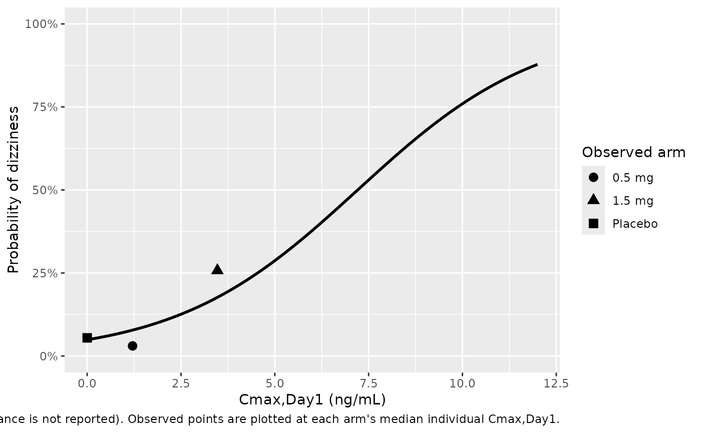
Figure 4 – exposure-response curve
curve_df <- tibble(CMAX = seq(0, 12, by = 0.05)) |>
  mutate(prob = dz_solve(CMAX))
#> Warning: There was 1 warning in `mutate()`.
#> ℹ In argument: `prob = dz_solve(CMAX)`.
#> Caused by warning:
#> ! multi-subject simulation without without 'omega'
observed <- tibble::tribble(
  ~arm, ~CMAX, ~events, ~n,
  "Placebo", 0, 6, 110,
  "0.5 mg", 1.21, 3, 99,
  "1.5 mg", 3.47, 26, 101
) |>
  mutate(rate = events / n)

ggplot(curve_df, aes(CMAX, prob)) +
  geom_line(linewidth = 1) +
  geom_point(data = observed, aes(CMAX, rate, shape = arm), size = 3) +
  scale_y_continuous(labels = scales::percent, limits = c(0, 1)) +
  labs(
    x = "Cmax,Day1 (ng/mL)", y = "Probability of dizziness", shape = "Observed arm",
    caption = paste(
      "Replicates the model curve of Figure 4 of Cosson 2018 (the 95% CI band is not",
      "reproduced: the intercept-slope covariance is not reported). Observed points",
      "are plotted at each arm's median individual Cmax,Day1."
    )
  )
Predicted incidence in the virtual cohort
er_arm <- bind_rows(
  tibble(treatment = "Placebo", CMAX = rep(0, n_per_arm)),
  cmax_day1 |> select(treatment, CMAX)
) |>
  mutate(prob = dz_solve(CMAX)) |>
  group_by(treatment) |>
  summarise(model_mean_pct = 100 * mean(prob), .groups = "drop") |>
  inner_join(
    tibble::tribble(
      ~treatment, ~paper_pred_pct, ~observed_pct,
      "Placebo", 100 * plogis(-2.970), 100 * 6 / 110,
      "0.5 mg", 9, 100 * 3 / 99,
      "1.5 mg", 24, 100 * 26 / 101
    ),
    by = "treatment"
  )
#> Warning: There was 1 warning in `mutate()`.
#> ℹ In argument: `prob = dz_solve(CMAX)`.
#> Caused by warning:
#> ! multi-subject simulation without without 'omega'
stopifnot(nrow(er_arm) == 3)
er_arm |>
  dplyr::rename(
    "Arm" = treatment,
    "Model, mean predicted (%)" = model_mean_pct,
    "Paper, predicted (%)" = paper_pred_pct,
    "Observed (%)" = observed_pct
  ) |>
knitr::kable(digits = 1, caption = "Dizziness incidence by arm. The paper's placebo prediction is the intercept alone; its active-arm predictions are from Results.")| Arm | Model, mean predicted (%) | Paper, predicted (%) | Observed (%) |
|---|---|---|---|
| 0.5 mg | 8.4 | 9.0 | 3.0 |
| 1.5 mg | 22.2 | 24.0 | 25.7 |
| Placebo | 4.9 | 4.9 | 5.5 |
p15 <- er_arm$model_mean_pct[er_arm$treatment == "1.5 mg"]
# Results quotes a 24% predicted risk at 1.5 mg. The mean over the cohort is
# robust to tail subjects; 15-35% still fails if the slope or Cmax scale is off.
stopifnot(p15 > 15, p15 < 35)
Assumptions and deviations
-
Asian relative bioavailability (Errata 1). The
covariate equation is printed as
F = 1 + 1.26 * ETHN, which would make Asian bioavailability 2.26 times the non-Asian value. Three other statements in the paper give a factor of 1.26: Table 1 lists the ethnicity effect on F as 1.26; Figure 2 shows Asian participants at -21% on every apparent parameter, which is 1/1.26 - 1; and the Discussion says that “Asians have slightly higher bioavailability (26%)”. The model uses 1.26 (fdepot = 1.26^RACE_ASIAN). Figure 3 is consistent with neither reading: its Asian curves are 1.26^2 = 1.588 times the matching non-Asian curves in every panel, which suggests that the simulation behind the figure applied the factor twice. The gate above confirms that every Asian curve in Figure 3 is exactly 1.26 times the model’s. -
Residual error scale (Errata 2). Table 1 lists
“Proportional residual error [% CV]” as 0.262 with an RSE of 0.831. A
0.26% proportional error is implausible for LC-MS/MS data pooled across
five trials. The value is read as a fraction (26.2% CV,
propSd = 0.262). A later simulation study by overlapping authors (Duvnjak 2024, doi:10.1002/psp4.13213), which built its scenarios from this model, uses a 26.4% proportional error, consistent with this reading. The “RSE 0.831” cannot be interpreted with confidence and is not used. - Figure 2 label (Errata 3). The Vc/F panel of Figure 2 labels a +40% symbol “Male”, but neither the equations nor Table 1 carry a sex effect on Vc/F. The symbol matches the smoking effect (+39.7%), and the panel has no other smoking symbol, so it is treated as a mislabel.
-
Signs of covariate effects. Table 1 prints the
ethnicity effect on fasted Ktr as 0.588 while the Ktr equation has
(1 - 0.588 * ETHN); the Discussion says absorption is delayed in Asian subjects. The model stores the signed coefficient -0.588 and applies(1 + e * RACE_ASIAN), matching the equation. The sex effects on Q/F and Vp/F are negative in both Table 1 and the equations. -
Between-subject variability. Table 1 reports BSV as
%CV for log-normal random effects without stating the conversion; the
variances use
omega^2 = log(CV^2 + 1). The six reported correlations among CL, Vc, Q and Vp form a positive-definite block. Ktr has separate fed and fasted random effects; the paper does not report correlations for them, so they are independent. There is no BSV on lag time (Results). - Absorption chain. “A chain of three compartments, including the depot compartment” is encoded as the depot plus two transit compartments, each emptying at Ktr into the next and the last into the central compartment, so the mean absorption time after the lag is 3/Ktr. The lag is applied to the depot. The Figure 3 match (peaks and troughs within 1%) supports this structure.
- Food-related Tmax delay. The model gives a fed-vs-fasted Day-1 Tmax delay of about 3.2 h; the Discussion quotes 2.5 h without saying how it was derived. The Day-1 Cmax reduction (about 30%) and the Figure 3 profiles match, so this is recorded rather than gated.
-
Covariate coding. The paper’s male indicator
SEXis stored as the canonicalSEXFand each sex effect is applied to1 - SEXF, so the female-reference typical values and coefficients are unchanged.FOOD,SMOKandETHNmap toFED,SMOKEandRACE_ASIANwithout value changes. Body weight effects are power functions normalised to 71 kg. - Virtual phase II cohort. The phase II covariate distribution is not published. The cohort uses the overall analysis-population sex and Asian shares, a log-normal weight matched to the 52 and 100 kg 5th and 95th percentiles, an assumed 25% smoking prevalence, and fed dosing.
-
Dizziness model residual. The logistic regression
has a Bernoulli likelihood and no residual error.
addSd_prob_dizzinessis a fixed placeholder of 0.001 so that the model has an observation statement; it is not from the paper. - Figure 4 confidence band. The band needs the intercept-slope covariance, which is not reported, so only the model curve is replicated.
- Supplement. The supporting information (goodness-of-fit plots, pcVPCs and weight-by-covariate distributions, Figures S1-S3) was not used; the main text carries the complete parameter set. No correction notice for this article was found (EuropePMC, checked 2026-10-11).