Vancomycin (Munir 2021)
Source:vignettes/articles/Munir_2021_vancomycin.Rmd
Munir_2021_vancomycin.RmdModel and source
- Citation: Munir MM, Rasheed H, Khokhar MI, Khan RR, Saeed HA, Abbas M, Ali M, Bilal R, Nawaz HA, Khan AM, Qamar S, Anjum SM, Usman M. Dose Tailoring of Vancomycin Through Population Pharmacokinetic Modeling Among Surgical Patients in Pakistan. Front Pharmacol. 2021;12:721819. doi:10.3389/fphar.2021.721819
- Description: One-compartment IV population PK model for vancomycin in 58 adult surgical patients in Pakistan (Munir 2021). Clearance carries linear, median-centred effects of raw Cockcroft-Gault creatinine clearance (increasing, reference 101.15 mL/min) and total body weight (decreasing as printed in Eq. 3, reference 75 kg); volume of distribution has no retained covariate. Additive residual error.
- Article: https://doi.org/10.3389/fphar.2021.721819 (open access, CC BY 4.0)
Population
Munir 2021 is a single-centre study at the surgical unit of Lahore General Hospital, Pakistan (August-December 2018). Fifty-eight adults (> 18 years) who had undergone a major surgical procedure and received intravenous vancomycin (0.5 h infusions of 500-1000 mg, most patients 1000 mg) contributed 176 plasma concentrations drawn after the first dose (average 3 per patient, range 1-7). Table 1 of the paper summarises the cohort: 39 male / 19 female, median age 54 years (25-86), median weight 75 kg (53-129), median serum creatinine 0.935 mg/dL (0.4-4.7) and median Cockcroft-Gault creatinine clearance 101.15 mL/min (15.9-177.2). The indications were grossly contaminated wounds, gas gangrene and severe peritonitis. Concentrations were measured by HPLC-UV (LLOQ 0.25 mg/L).
The same information is available programmatically via the model’s
population metadata
(readModelDb("Munir_2021_vancomycin")()$population).
Source trace
The per-parameter origin is recorded as an in-file comment next to
each ini() entry in
inst/modeldb/specificDrugs/Munir_2021_vancomycin.R. The
table below collects them in one place for review.
| Equation / parameter | Value | Source location |
|---|---|---|
lcl (CL at CRCL = 101.15 mL/min, WT = 75 kg) |
log(2.45) L/h |
Table 2, row CL (L/h) (RSE 2%), footnote b; Eq. 1
constant |
lvc (volume of distribution) |
log(22.6) L |
Table 2, row V (L) (RSE 5%) |
e_crcl_cl (linear CRCL slope on CL) |
0.0046 per mL/min |
Table 2, row CL-CRCL (RSE 13%); Eq. 2 |
e_wt_cl (linear WT slope on CL) |
-0.011 per kg |
Table 2, row CL-WT = 0.011 (RSE 10%); sign from Eq.
3 |
etalcl (IIV variance on CL) |
log(1 + 0.113^2) = 0.012688 |
Table 2, row BSV-CL (%) = 11.3, footnote e (percent
CV) |
etalvc (IIV variance on V) |
log(1 + 0.228^2) = 0.050668 |
Table 2, row BSV-Vd (%) = 22.8, footnote e (percent
CV) |
addSd (additive residual SD) |
3.07 mg/L |
Table 2, row Additive error; Results, Population PK
modeling |
| CL model | cl <- exp(lcl + etalcl) * (1 + e_crcl_cl*(CRCL - 101.15)) * (1 + e_wt_cl*(WT - 75)) |
Eqs. 1-3 |
| Structure (one compartment, first-order elimination) | n/a | Results, Population PK modeling: “one-compartment model with first-order elimination (ADVAN1 TRANS2)” |
| Centring values 101.15 mL/min and 75 kg | n/a | Text below Eq. 3: the cohort medians; also Table 1 |
Virtual cohort and simulation
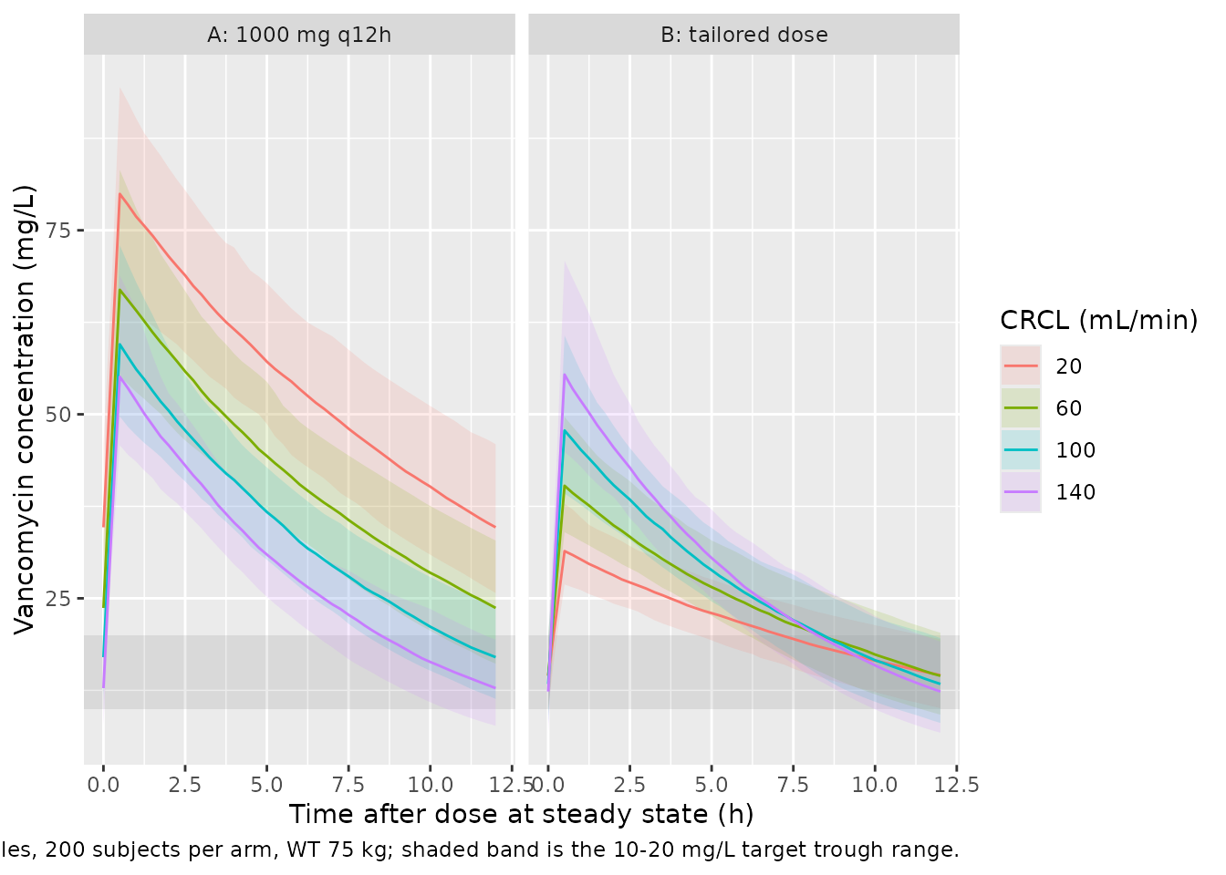
The paper’s dosing simulations (Methods, Dosing simulations; Table 3) use four virtual patients with CRCL 20, 60, 100 and 140 mL/min, each given the same 1000 mg q12h and then a tailored dose (400, 600, 800 and 1000 mg q12h), and report the steady-state trough as mean +/- SD over 1000 simulated subjects per arm. The body weight of those virtual patients is not stated; the cohort median 75 kg is used here, which makes the weight factor exactly 1. The 0.5 h infusion is the study infusion duration. Each arm below has 200 subjects dosed q12h for 20 doses (240 h, more than 20 typical half-lives even at CRCL 20 mL/min), and the last dosing interval is observed.
# `set.seed()` seeds R's RNG only; rxode2's own simulation streams depend on the
# solver thread count, so every cohort assertion below is written to hold for
# any cohort the model can produce.
set.seed(20211111)
n_per_arm <- 200L # cap is 200 per arm
t_inf <- 0.5
tau <- 12
n_dose <- 20L
t_last <- (n_dose - 1L) * tau # time of the last dose

# Table 3 of Munir 2021.
arms <- tibble::tribble(
  ~CRCL, ~regimen,   ~amt, ~paper_mean, ~paper_sd,
  20,    "same",     1000, 33.3,        7.54,
  60,    "same",     1000, 23.9,        5.73,
  100,   "same",     1000, 18.0,        4.56,
  140,   "same",     1000, 13.7,        3.79,
  20,    "tailored",  400, 13.3,        3.01,
  60,    "tailored",  600, 14.4,        3.44,
  100,   "tailored",  800, 14.4,        3.65,
  140,   "tailored", 1000, 13.7,        3.79
) |>
  dplyr::mutate(
    arm = sprintf("CRCL %d, %s %d mg", CRCL, regimen, amt),
    arm_no = dplyr::row_number()
  )

obs_times <- unique(round(c(seq(t_last, t_last + tau, by = 0.25)), 9))

make_arm <- function(i) {
  a <- arms[i, ]
  ids <- (a$arm_no - 1L) * n_per_arm + seq_len(n_per_arm)
  dosing <- tidyr::crossing(id = ids, dose_no = seq_len(n_dose) - 1L) |>
    dplyr::mutate(
      time = dose_no * tau, amt = a$amt, evid = 1L, dur = t_inf,
      cmt = "central"
    ) |>
    dplyr::select(-dose_no)
  obs <- tidyr::crossing(id = ids, time = obs_times) |>
    dplyr::mutate(amt = NA_real_, evid = 0L, dur = NA_real_, cmt = "central")
  dplyr::bind_rows(dosing, obs) |>
    dplyr::mutate(CRCL = a$CRCL, WT = 75, arm = a$arm)
}

events <- dplyr::bind_rows(lapply(seq_len(nrow(arms)), make_arm)) |>
  dplyr::arrange(id, time, dplyr::desc(evid))

stopifnot(dplyr::n_distinct(events$id) == n_per_arm * nrow(arms))
mod <- readModelDb("Munir_2021_vancomycin")

sim <- rxode2::rxSolve(
  mod,
  events = events,
  keep = c("arm", "CRCL", "WT"),
  useLinCmt = FALSE
) |>
  as.data.frame()
#> ℹ parameter labels from comments will be replaced by 'label()'

stopifnot(nrow(sim) > 0L, !all(is.na(sim$Cc)))
Replicate published figures
Figure 1B – clearance versus creatinine clearance
# Replicates Figure 1B of Munir 2021 (CL vs CRCL). The line is the typical-value
# relationship at WT = 75 kg; the points are individual clearances for a cohort
# spanning the observed CRCL range.
cl_line <- tibble::tibble(CRCL = seq(15, 180, by = 1)) |>
  dplyr::mutate(cl = 2.45 * (1 + 0.0046 * (CRCL - 101.15)))

ggplot(cl_line, aes(CRCL, cl)) +
  geom_line(colour = "firebrick", linewidth = 1) +
  labs(
    x = "Creatinine clearance (mL/min)", y = "Vancomycin CL (L/h)",
    title = "Figure 1B -- clearance increases with creatinine clearance",
    caption = paste(
      "Replicates the relationship in Figure 1B of Munir 2021:",
      "CL = 2.45 x (1 + 0.0046 x (CRCL - 101.15)) at 75 kg (Eqs. 1-3)."
    )
  )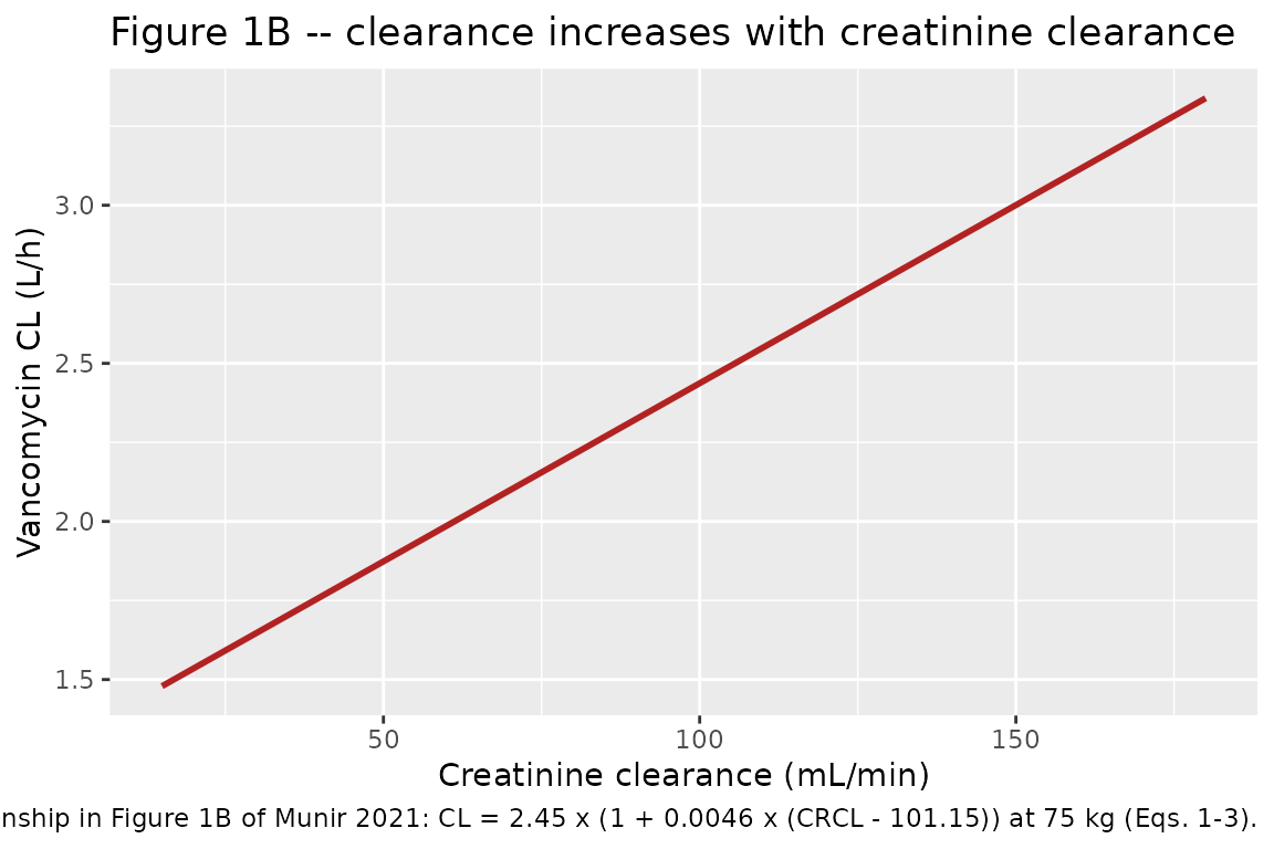
Figure 5 – steady-state profiles, common and tailored doses
# Replicates Figure 5A (1000 mg q12h) and 5B (tailored doses) of Munir 2021.
sim |>
  dplyr::filter(time >= t_last) |>
  dplyr::mutate(
    tad = time - t_last,
    panel = ifelse(grepl("same", arm), "A: 1000 mg q12h", "B: tailored dose"),
    CRCL = factor(CRCL)
  ) |>
  dplyr::group_by(panel, CRCL, tad) |>
  dplyr::summarise(
    Q05 = quantile(Cc, 0.05), Q50 = median(Cc), Q95 = quantile(Cc, 0.95),
    .groups = "drop"
  ) |>
  ggplot(aes(tad, Q50, colour = CRCL, fill = CRCL)) +
  annotate(
    "rect",
    xmin = -Inf, xmax = Inf, ymin = 10, ymax = 20, alpha = 0.12
  ) +
  geom_ribbon(aes(ymin = Q05, ymax = Q95), alpha = 0.15, colour = NA) +
  geom_line() +
  facet_wrap(~panel) +
  labs(
    x = "Time after dose at steady state (h)",
    y = "Vancomycin concentration (mg/L)",
    colour = "CRCL (mL/min)", fill = "CRCL (mL/min)",
    caption = paste(
      "Replicates Figure 5 of Munir 2021. Median and 5th-95th percentiles,",
      "200 subjects per arm, WT 75 kg; shaded band is the 10-20 mg/L target",
      "trough range."
    )
  )
Deterministic structural checks
These compare the packaged model against the paper’s equations for a typical subject with the random effects zeroed. Both sides use the same parameters, so the tolerances are tight.
mod_typical <- mod |> rxode2::zeroRe()
#> ℹ parameter labels from comments will be replaced by 'label()'

grid <- tidyr::crossing(CRCL = c(20, 60, 101.15, 140), WT = c(53, 75, 129)) |>
  dplyr::mutate(id = dplyr::row_number())
ev_cl <- dplyr::bind_rows(
  dplyr::mutate(
    grid,
    time = 0, amt = 1000, evid = 1L, dur = t_inf, cmt = "central"
  ),
  dplyr::mutate(
    grid,
    time = 1, amt = NA_real_, evid = 0L, dur = NA_real_, cmt = "central"
  )
)
cl_check <- rxode2::rxSolve(
  mod_typical, ev_cl,
  keep = c("CRCL", "WT"), returnType = "data.frame", useLinCmt = FALSE
) |>
  dplyr::distinct(id, CRCL, WT, cl, vc) |>
  dplyr::mutate(
    cl_eq = 2.45 * (1 + 0.0046 * (CRCL - 101.15)) * (1 - 0.011 * (WT - 75)),
    rel = abs(cl - cl_eq) / cl_eq
  )
#> ℹ omega/sigma items treated as zero: 'etalcl', 'etalvc'
#> Warning: multi-subject simulation without without 'omega'

stopifnot(nrow(cl_check) == nrow(grid))
stopifnot(max(cl_check$rel) < 1e-8, max(abs(cl_check$vc - 22.6)) < 1e-8)
# Eq. 3 as printed: clearance FALLS with body weight.
stopifnot(
  cl_check$cl[cl_check$CRCL == 101.15 & cl_check$WT == 53] >
    cl_check$cl[cl_check$CRCL == 101.15 & cl_check$WT == 129]
)

cl_check |>
  dplyr::select(CRCL, WT, cl, cl_eq) |>
  dplyr::rename(
    "CRCL (mL/min)" = CRCL, "WT (kg)" = WT,
    "Model CL (L/h)" = cl, "Eqs. 1-3 CL (L/h)" = cl_eq
  ) |>
knitr::kable(digits = 4, caption = "Model clearance reproduces Eqs. 1-3.")| CRCL (mL/min) | WT (kg) | Model CL (L/h) | Eqs. 1-3 CL (L/h) |
|---|---|---|---|
| 20.00 | 53 | 1.9070 | 1.9070 |
| 20.00 | 75 | 1.5354 | 1.5354 |
| 20.00 | 129 | 0.6234 | 0.6234 |
| 60.00 | 53 | 2.4669 | 2.4669 |
| 60.00 | 75 | 1.9862 | 1.9862 |
| 60.00 | 129 | 0.8064 | 0.8064 |
| 101.15 | 53 | 3.0429 | 3.0429 |
| 101.15 | 75 | 2.4500 | 2.4500 |
| 101.15 | 129 | 0.9947 | 0.9947 |
| 140.00 | 53 | 3.5867 | 3.5867 |
| 140.00 | 75 | 2.8878 | 2.8878 |
| 140.00 | 129 | 1.1725 | 1.1725 |
# Closed-form steady-state trough for a q12h 0.5 h infusion, one compartment.
trough_ss <- function(amt, cl, vc) {
  k <- cl / vc
  (amt / (t_inf * cl)) * (1 - exp(-k * t_inf)) * exp(-k * (tau - t_inf)) /
    (1 - exp(-k * tau))
}

typ <- arms |>
  dplyr::rowwise() |>
  dplyr::mutate(
    cl_typ = 2.45 * (1 + 0.0046 * (CRCL - 101.15)),
    closed_form = trough_ss(amt, cl_typ, 22.6),
    solved = {
      ev <- rxode2::et(
        amt = amt, dur = t_inf, ii = tau, addl = n_dose - 1L, cmt = "central"
      ) |>
        rxode2::et(time = n_dose * tau, cmt = "central") |>
        as.data.frame()
      ev$CRCL <- CRCL
      ev$WT <- 75
      s <- rxode2::rxSolve(
        mod_typical, ev,
        returnType = "data.frame", useLinCmt = FALSE
      )
      s$Cc[abs(s$time - n_dose * tau) < 1e-8][1]
    }
  ) |>
  dplyr::ungroup() |>
  dplyr::mutate(pct_diff = 100 * (solved - closed_form) / closed_form)
#> ℹ omega/sigma items treated as zero: 'etalcl', 'etalvc'
#> ℹ omega/sigma items treated as zero: 'etalcl', 'etalvc'
#> ℹ omega/sigma items treated as zero: 'etalcl', 'etalvc'
#> ℹ omega/sigma items treated as zero: 'etalcl', 'etalvc'
#> ℹ omega/sigma items treated as zero: 'etalcl', 'etalvc'
#> ℹ omega/sigma items treated as zero: 'etalcl', 'etalvc'
#> ℹ omega/sigma items treated as zero: 'etalcl', 'etalvc'
#> ℹ omega/sigma items treated as zero: 'etalcl', 'etalvc'

# 20 doses reach steady state to well under 0.1% at the slowest elimination.
stopifnot(!anyNA(typ$solved), max(abs(typ$pct_diff)) < 0.1)

typ |>
  dplyr::select(arm, closed_form, solved) |>
  dplyr::rename(
    "Arm" = arm,
    "Closed-form SS trough (mg/L)" = closed_form,
    "rxode2 trough after 20 doses (mg/L)" = solved
  ) |>
knitr::kable(digits = 3, caption = "Typical-subject steady-state troughs.")| Arm | Closed-form SS trough (mg/L) | rxode2 trough after 20 doses (mg/L) |
|---|---|---|
| CRCL 20, same 1000 mg | 35.726 | 35.726 |
| CRCL 60, same 1000 mg | 24.177 | 24.177 |
| CRCL 100, same 1000 mg | 17.173 | 17.173 |
| CRCL 140, same 1000 mg | 12.574 | 12.574 |
| CRCL 20, tailored 400 mg | 14.290 | 14.290 |
| CRCL 60, tailored 600 mg | 14.506 | 14.506 |
| CRCL 100, tailored 800 mg | 13.738 | 13.738 |
| CRCL 140, tailored 1000 mg | 12.574 | 12.574 |
PKNCA validation
PKNCA is run over the last (steady-state) dosing interval, re-based so the last dose sits at time 0. The interval end-point concentration is the trough the paper reports in Table 3.
sim_nca <- sim |>
  dplyr::filter(!is.na(Cc), time >= t_last) |>
  dplyr::mutate(time_rel = round(time - t_last, 9)) |>
  dplyr::select(id, time_rel, Cc, arm)

conc_obj <- PKNCA::PKNCAconc(as.data.frame(sim_nca), Cc ~ time_rel | arm + id)

dose_df <- sim_nca |>
  dplyr::distinct(id, arm) |>
  dplyr::left_join(dplyr::select(arms, arm, amt), by = "arm") |>
  dplyr::mutate(time_rel = 0) |>
  as.data.frame()
dose_obj <- PKNCA::PKNCAdose(dose_df, amt ~ time_rel | arm + id)

intervals <- data.frame(
  start = 0, end = tau,
  ctrough = TRUE, cmax = TRUE, tmax = TRUE, auclast = TRUE, cav = TRUE
)

nca_res <- PKNCA::pk.nca(
  PKNCA::PKNCAdata(conc_obj, dose_obj, intervals = intervals)
)

nca_wide <- as.data.frame(nca_res) |>
  dplyr::filter(PPTESTCD %in% c("ctrough", "cmax", "tmax", "auclast", "cav")) |>
  dplyr::select(arm, id, PPTESTCD, PPORRES) |>
  tidyr::pivot_wider(names_from = PPTESTCD, values_from = PPORRES)

stopifnot(nrow(nca_wide) == n_per_arm * nrow(arms))
stopifnot(!anyNA(nca_wide$ctrough), !anyNA(nca_wide$auclast))

nca_wide |>
  dplyr::group_by(arm) |>
  dplyr::summarise(
    cmax = median(cmax), auclast = median(auclast),
    cav = median(cav), ctrough = median(ctrough),
    .groups = "drop"
  ) |>
  dplyr::left_join(dplyr::select(arms, arm, arm_no), by = "arm") |>
  dplyr::arrange(arm_no) |>
  dplyr::select(-arm_no) |>
  dplyr::rename(
    "Arm" = arm, "Cmax (mg/L)" = cmax, "AUCtau (mg*h/L)" = auclast,
    "Cav (mg/L)" = cav, "Ctrough (mg/L)" = ctrough
  ) |>
  knitr::kable(
    digits = 2,
    caption = "Median steady-state NCA over one 12 h interval, by arm."
)| Arm | Cmax (mg/L) | AUCtau (mg*h/L) | Cav (mg/L) | Ctrough (mg/L) |
|---|---|---|---|---|
| CRCL 20, same 1000 mg | 79.94 | 648.77 | 54.06 | 34.65 |
| CRCL 60, same 1000 mg | 66.92 | 499.20 | 41.60 | 23.69 |
| CRCL 100, same 1000 mg | 59.51 | 413.21 | 34.43 | 17.00 |
| CRCL 140, same 1000 mg | 55.09 | 349.68 | 29.14 | 12.80 |
| CRCL 20, tailored 400 mg | 31.41 | 261.30 | 21.77 | 14.56 |
| CRCL 60, tailored 600 mg | 40.30 | 300.12 | 25.01 | 14.47 |
| CRCL 100, tailored 800 mg | 47.80 | 324.44 | 27.04 | 13.36 |
| CRCL 140, tailored 1000 mg | 55.40 | 346.72 | 28.89 | 12.34 |
Steady-state dose recovery
At steady state CL * AUCtau / Dose = 1. Checked on each
subject’s own clearance, so the only error source is trapezoidal
integration on the 0.25 h grid.
recovery <- nca_wide |>
  dplyr::left_join(
    sim |> dplyr::distinct(id, cl),
    by = "id"
  ) |>
  dplyr::left_join(dplyr::select(arms, arm, amt), by = "arm") |>
  dplyr::mutate(recovery = cl * auclast / amt)

# Linear-trapezoid error on a 0.25 h grid over a 0.5 h infusion peak is a
# fraction of a percent; a unit or volume error would move this by far more.
stopifnot(abs(median(recovery$recovery) - 1) < 0.01)
stopifnot(quantile(abs(recovery$recovery - 1), 0.9) < 0.02)
Comparison against the published simulation (Table 3)
Table 3 reports the simulated steady-state trough as mean +/-
SD, so the comparison below uses the simulated mean and SD
rather than ncaComparisonTable() (which pools by median).
Two features of Table 3 are worth noting. First, the tailored-dose rows
are the same-dose rows scaled exactly by the dose ratio (e.g. 33.3 x 0.4
= 13.3 and 7.54 x 0.4 = 3.01), so the published troughs are individual
predictions without the additive residual error, which would not scale
with dose; the model’s Cc (without residual error) is
therefore the right comparator. Second, the published SDs pin the scale
of the Table 2 BSV entries: reading 11.3% and 22.8% as coefficients of
variation reproduces them, while reading them as variances (0.113 and
0.228) would inflate the trough SD roughly three-fold.
tab3 <- nca_wide |>
  dplyr::group_by(arm) |>
  dplyr::summarise(
    sim_mean = mean(ctrough), sim_sd = sd(ctrough), .groups = "drop"
  ) |>
  dplyr::left_join(arms, by = "arm") |>
  dplyr::arrange(arm_no) |>
  dplyr::mutate(
    pct_diff_mean = 100 * (sim_mean - paper_mean) / paper_mean,
    sd_ratio = sim_sd / paper_sd
  )

tab3 |>
  dplyr::select(
    arm, paper_mean, sim_mean, pct_diff_mean, paper_sd, sim_sd, sd_ratio
  ) |>
  dplyr::rename(
    "Arm" = arm,
    "Published mean (mg/L)" = paper_mean,
    "Simulated mean (mg/L)" = sim_mean,
    "Mean % diff" = pct_diff_mean,
    "Published SD" = paper_sd,
    "Simulated SD" = sim_sd,
    "SD ratio" = sd_ratio
  ) |>
  knitr::kable(
    digits = 2,
    caption = "Steady-state trough versus Munir 2021 Table 3."
)| Arm | Published mean (mg/L) | Simulated mean (mg/L) | Mean % diff | Published SD | Simulated SD | SD ratio |
|---|---|---|---|---|---|---|
| CRCL 20, same 1000 mg | 33.3 | 35.56 | 6.77 | 7.54 | 6.87 | 0.91 |
| CRCL 60, same 1000 mg | 23.9 | 23.89 | -0.05 | 5.73 | 5.30 | 0.92 |
| CRCL 100, same 1000 mg | 18.0 | 17.38 | -3.43 | 4.56 | 4.18 | 0.92 |
| CRCL 140, same 1000 mg | 13.7 | 12.99 | -5.21 | 3.79 | 3.69 | 0.97 |
| CRCL 20, tailored 400 mg | 13.3 | 14.48 | 8.90 | 3.01 | 2.95 | 0.98 |
| CRCL 60, tailored 600 mg | 14.4 | 14.51 | 0.78 | 3.44 | 3.14 | 0.91 |
| CRCL 100, tailored 800 mg | 14.4 | 13.67 | -5.04 | 3.65 | 3.38 | 0.93 |
| CRCL 140, tailored 1000 mg | 13.7 | 12.53 | -8.54 | 3.79 | 3.81 | 1.01 |
# Centre and envelope only (never the extremes of one cohort). The typical-value
# troughs differ from Table 3 by +7.3 / +1.2 / -4.6 / -8.2% at CRCL
# 20 / 60 / 100 / 140 (see Assumptions and deviations), so the envelope sits
# at 15%. A mis-transcribed CL, V, dose or unit moves every arm by tens of
# percent; reading BSV as variance would make the SD ratio about 3.
stopifnot(
  abs(median(tab3$pct_diff_mean)) < 7,
  max(abs(tab3$pct_diff_mean)) < 15,
  median(tab3$sd_ratio) > 0.75, median(tab3$sd_ratio) < 1.33
)
Assumptions and deviations
-
Sign of the weight effect. Table 2 lists
CL-WT = 0.011without a sign and footnote d calls it the “proportional change in CL with weight”, but Eq. 3 printsCLWT = (1 - 0.011 x (WT - 75))(the minus sign is present in both the typeset PDF and the article’s MathML). The printed equation is followed, so clearance falls by 1.1% per kg above 75 kg. The factor is 1.24 at the lightest patient (53 kg) and 0.41 at the heaviest (129 kg), and it reaches zero at 165.9 kg: the model must not be used outside the observed 53-129 kg range. The paper does not discuss the direction of the effect. - Residual error model. The Results paragraph on population PK modelling says residual variability “was described by a proportional error model” and, two sentences later, that “the additive error was 3.07”; Table 2 labels the same 3.07 “Additive error”. The value is encoded as an additive SD in mg/L. Read as a proportional error it would be either 307% (as a fraction) or 3.07% (as a percentage), both implausible for an HPLC assay with 17.8% inter-day precision, and the DV-versus-IPRED panel of Figure 3B shows a roughly constant scatter of a few mg/L across the 5-50 mg/L range. Whether 3.07 is an SD or a variance is not stated; it is read as an SD.
- BSV values in the text. The Results text gives BSV-CL as 9.14% (after covariates) and the Discussion gives BSV-Vd as 16.1%; Table 2 gives 11.3% and 22.8%. The Table 2 final estimates are used, and the Table 3 trough SDs are reproduced with them (above).
- Table 3 means. Typical-value steady-state troughs from Eqs. 1-3 differ from the Table 3 means by +7.3, +1.2, -4.6 and -8.2% at CRCL 20, 60, 100 and 140 mL/min. The pattern (too high at low CRCL, too low at high CRCL) is not explained by the unstated weight of the virtual patients (the weight factor is a uniform multiplier) or by a 1 h instead of 0.5 h infusion. The paper does not print its simulation settings beyond CRCL, dose and interval; the published parameters are used unchanged.
- Virtual patients. Weight is set to the cohort median 75 kg in the dosing simulations, and the 0.5 h study infusion duration is used; neither is stated for the paper’s Table 3 simulations.
-
Table 1 percentages. Table 1 prints 39 male (73.7%)
/ 19 female (26.3%) and patient-type percentages that sum over 38
patients, not 58. The counts are used; the model’s
population$sex_female_pctis 19/58 = 32.8%. - CRCL normalisation. Cockcroft-Gault creatinine clearance is used in raw mL/min, as the paper describes no BSA normalisation.