Aditoprim PBPK/PD against Streptococcus suis in swine (Mi 2024)

Model and source

Mi 2024 builds a physiologically based pharmacokinetic / pharmacodynamic (PBPK/PD) model for aditoprim (ADP), a veterinary diaminopyrimidine, in swine. The paper has two applications: choosing an intramuscular dosage regimen that clears Streptococcus suis without selecting for resistance, and predicting the withdrawal interval needed to bring edible-tissue residues below their maximum residue limits.

Two models are packaged, mirroring the two layers the authors fitted separately:

• Mi_2024_aditoprim_pbpk – the whole-body swine PBPK model on its own, calibrated and validated against tissue residue data and used for the withdrawal-interval assessment.
• Mi_2024_aditoprim_pbpkpd – that PBPK model coupled to the two-subpopulation semi-mechanistic PD model, used for dosage optimisation.

pbpk <- readModelDb("Mi_2024_aditoprim_pbpk")
pkpd <- readModelDb("Mi_2024_aditoprim_pbpkpd")

• Citation: Mi K, Sun L, Zhang L, Tang A, Tian X, Hou Y, Sun L, Huang L. A physiologically based pharmacokinetic/pharmacodynamic model to determine dosage regimens and withdrawal intervals of aditoprim against Streptococcus suis. Front Pharmacol. 2024;15:1378034. doi:10.3389/fphar.2024.1378034. Model equations transcribed from Supplementary Material section 3.1 (Berkeley Madonna code) and Supplementary Table 3; final parameter values from Table 2; Monte Carlo distributions from Table 3.
• Article: https://doi.org/10.3389/fphar.2024.1378034
• Supplement (equations, Berkeley Madonna and Monolix code, residue tables): https://www.frontiersin.org/articles/10.3389/fphar.2024.1378034/full#supplementary-material

Population

No animals were dosed for this modelling paper. The PBPK layer was calibrated and validated against four previously published swine datasets (Mi 2024 Table 1), with graphical data digitised using WebPlotDigitizer 3.10:

• Calibration – Wang et al. (2022) plasma after a single 5 mg/kg intramuscular (IM) dose (n = 6), and Wang (2020) liver, kidney, muscle and fat after 10 mg/kg every 12 h for 14 doses (n = 40).
• Validation – Qu et al. (2022) plasma after a single 5 mg/kg IM dose (n = 6), and Wang (2016) liver, kidney, muscle and fat after 5 mg/kg every 24 h for 7 doses (n = 40).

The tissue concentrations behind the two residue-depletion datasets are reproduced in Supplementary Tables 1 and 2 and are used as the validation target below. Physiological parameters are literature swine values (Upton 2008); the model reference body weight is 30 kg.

The PD layer is independent of that swine population: it was fitted by non-linear mixed effects in Monolix 2018R1 to in vitro time-killing curves of ADP against S. suis ATCC 49619 run in triplicate, with the MIC determined per CLSI 2018 as 0.5 ug/mL. The integrated model is therefore an in silico projection (performed by the authors in Mlxplore 2018a), not a model observed in any single cohort.

The same information is available programmatically via readModelDb("Mi_2024_aditoprim_pbpk")()$population.

Source trace

Every ini() entry carries an in-file comment naming its source location. The table below collects them, and flags the values that are not in the main paper.

Equation / parameter	Value	Source location
Body weight BW	30 kg	Table 2; Suppl 3.1 BW=30
Cardiac output QCC	4.944 L/h/kg	Table 2 (Upton 2008)
Liver blood flow QLC	0.3053 of QCC	Table 2
Kidney blood flow QKC	0.1398 of QCC	Table 2
Muscle blood flow QMC	0.2524 of QCC	Table 2
Fat blood flow QFC	0.1747 of QCC	Suppl 3.1 QFC=0.1747 only – absent from Table 2
Rest-of-body blood flow	0.1278 of QCC (complement)	Suppl 3.1 QOT=QC-(QL+QK+QM+QF)
Liver volume VLC	0.0294 of BW	Table 2
Kidney volume VKC	0.004 of BW	Table 2
Muscle volume VMC	0.4 of BW	Table 2
Fat volume VFC	0.3 of BW	Suppl 3.1 VFC=0.3 only – absent from Table 2
Blood volume VBC	0.06 of BW	Suppl 3.1 VBC=0.06; = Table 2 VartC 0.016 + VvenC 0.044
Rest-of-body volume	0.2066 of BW (complement)	Suppl 3.1 VOT=BW-(VL+VK+VM+VF+Vblood)
Liver partition PL	5.249	Table 2 (Calculated/optimized)
Kidney partition PK	6	Table 2 (Calculated/optimized)
Muscle partition PM	0.79	Table 2 (Calculated/optimized)
Fat partition PF	1.1	Table 2 (Calculated/optimized)
Rest partition PT	0.18	Table 2 (Calculated/optimized)
IM absorption Kim	1.3 /h	Table 2 (Model fitting)
Fast-absorption fraction Frac	0.92	Table 2 (Model fitting)
Dissolution Kdiss	0.0118 /h	Table 2 (Model fitting)
Hepatic clearance KML	0.01 L/h/kg	Table 2 (Model fitting)
Renal clearance KurineC	0.1 L/h/kg	Table 2 (Model fitting)
Plasma protein binding PB	0.82 bound	Table 2 (Model fitting); Suppl 3.1 CAfree = CA*(1-PB)
Monte Carlo distributions	lognormal, CV 0.40 (0.10 for Frac)	Table 3
PBPK ODE system	n/a	Suppl Table 3 and Suppl 3.1 (Berkeley Madonna code)
Growth rate Kgrowth	0.833 /h	Table 4
Stationary-phase count Bmax	4.61e7 CFU/mL	Table 4
Maximum kill rate Emax	1.45 /h	Table 4
Susceptible potency EC50_S	0.685 mg/L	Table 4
Resistant potency EC50_R	1.63 mg/L	Table 4
Hill coefficient gamma	2.5	Table 4
Mutation frequency MF	1e-3 (fixed)	Table 4
Starting inoculum	1e5 CFU/mL split by MF	Suppl 3.2 E_0 =99900, R_0=100
MIC	0.5 ug/mL	Section 3.4 (CLSI 2018)
PD ODE system	n/a	Eq 2-3, corrected against Suppl 3.2 Monolix code (see Errata E1)
Liver MRL	0.303 ug/g	Section 2.7.3 (Wang et al. 2016)
Kidney MRL	0.084 ug/g	Section 2.7.3 (Wang et al. 2016)

Monte Carlo parameterisation

Mi 2024 Table 3 gives a mean, a CV and 2.5 / 97.5 percentile bounds for each of the seven parameters carried through the Monte Carlo analysis. Those bounds identify the parameterisation exactly: each is lognormal with arithmetic mean equal to the Table 2 point estimate, so the log-scale variance is log(1 + CV^2). The check below reproduces all seven pairs of printed bounds.

mc <- tibble::tribble(
  ~parameter, ~mean,  ~cv,  ~lower_pub, ~upper_pub,
  "PL",        5.249, 0.40, 2.29,       10.37,
  "PK",        6.00,  0.40, 2.62,       11.85,
  "PM",        0.79,  0.40, 0.34,        1.56,
  "PF",        1.10,  0.40, 0.48,        2.17,
  "KurineC",   0.10,  0.40, 0.04,        0.20,
  "Frac",      0.92,  0.10, 0.75,        1.00,
  "PB",        0.82,  0.40, 0.36,        0.99
) |>
  mutate(
    var_log   = log(1 + cv^2),
    mu_log    = log(mean) - var_log / 2,
    lower_fit = exp(mu_log - qnorm(0.975) * sqrt(var_log)),
    upper_fit = exp(mu_log + qnorm(0.975) * sqrt(var_log))
  )

mc |>
  mutate(across(c(var_log, lower_fit, upper_fit), \(x) round(x, 4))) |>
  select(parameter, mean, cv, var_log, lower_pub, lower_fit, upper_pub, upper_fit) |>
  dplyr::rename(
    "Parameter"          = parameter,
    "Mean"               = mean,
    "CV"                 = cv,
    "log(1 + CV^2)"      = var_log,
    "Lower (Table 3)"    = lower_pub,
    "Lower (derived)"    = lower_fit,
    "Upper (Table 3)"    = upper_pub,
    "Upper (derived)"    = upper_fit
  ) |>
  knitr::kable(caption = "Mi 2024 Table 3 bounds reproduced by a lognormal with arithmetic mean equal to the Table 2 estimate. Frac and PB are fractions and their published upper bounds are truncated at 1.00 and 0.99.")

Mi 2024 Table 3 bounds reproduced by a lognormal with arithmetic mean equal to the Table 2 estimate. Frac and PB are fractions and their published upper bounds are truncated at 1.00 and 0.99.

Parameter	Mean	CV	log(1 + CV^2)	Lower (Table 3)	Lower (derived)	Upper (Table 3)	Upper (derived)
PL	5.249	0.4	0.1484	2.29	2.2904	10.37	10.3699
PK	6.000	0.4	0.1484	2.62	2.6181	11.85	11.8536
PM	0.790	0.4	0.1484	0.34	0.3447	1.56	1.5607
PF	1.100	0.4	0.1484	0.48	0.4800	2.17	2.1732
KurineC	0.100	0.4	0.1484	0.04	0.0436	0.20	0.1976
Frac	0.920	0.1	0.0100	0.75	0.7529	1.00	1.1131
PB	0.820	0.4	0.1484	0.36	0.3578	0.99	1.6200

Virtual cohort and simulation set-up

All simulations use the 30 kg reference pig of Table 2. Cohorts are capped at 200 animals per arm; Mi 2024 used 1000 (see Errata E6).

set.seed(20240417)
BW <- 30

# Build an IM regimen. The dose is split between the fast injection-site pool
# (`depot`) and the slow-release depot (`depot2`) by the model's own
# bioavailability terms, so the same amount is dosed to both compartments.
make_events <- function(dose_mg_per_kg, ii, n_doses, obs_times, n = 1L,
                        id_offset = 0L, label = NA_character_) {
  amt <- dose_mg_per_kg * BW
  dose_rows <- tidyr::expand_grid(
    id  = id_offset + seq_len(n),
    cmt = c("depot", "depot2"),
    time = ii * (seq_len(n_doses) - 1L)
  ) |>
    mutate(amt = amt, evid = 1L)
  obs_rows <- tidyr::expand_grid(
    id = id_offset + seq_len(n),
    time = obs_times
  ) |>
    # Observation rows point at an ODE STATE (`blood`), never at an
    # algebraic observable such as `Cc`.
    mutate(cmt = "blood", amt = NA_real_, evid = 0L)
  bind_rows(dose_rows, obs_rows) |>
    mutate(WT = BW, regimen = label) |>
    arrange(id, time, desc(evid))
}

Replicating the PBPK layer (Figures 2 and 3)

Mi 2024 Figures 2 and 3 compare predicted and observed tissue concentrations for the calibration and validation regimens. The observed values are tabulated in Supplementary Tables 1 and 2, which lets the comparison be quantitative rather than visual.

pbpk_typ <- pbpk |> rxode2::zeroRe()

sim_tissue <- function(dose, ii, n_doses, horizon_d) {
  ev <- make_events(dose, ii, n_doses, obs_times = seq(0, horizon_d * 24, by = 1))
  rxode2::rxSolve(pbpk_typ, events = ev, omega = NA, returnType = "data.frame")
}

# Calibration: 10 mg/kg q12h x 14 doses (Wang 2020; Suppl Table 1)
cal <- sim_tissue(10, 12, 14, 30)
t_last_cal <- 12 * 13

# Validation: 5 mg/kg q24h x 7 doses (Wang 2016; Suppl Table 2)
val <- sim_tissue(5, 24, 7, 30)
t_last_val <- 24 * 6

observed <- bind_rows(
  tibble::tribble(
    ~dataset, ~day, ~Liver, ~Kidney, ~Muscle, ~Fat,
    "Calibration (10 mg/kg q12h x 14)", 0.5, 13311.0, 29283.5, 3439.1, 2524.7,
    "Calibration (10 mg/kg q12h x 14)", 3.0,  1305.4,  2709.6,  302.6,  347.9,
    "Calibration (10 mg/kg q12h x 14)", 7.0,   255.7,   308.5,   69.7,   82.4,
    "Calibration (10 mg/kg q12h x 14)", 14.0,   90.4,    77.7,     NA,     NA
  ),
  tibble::tribble(
    ~dataset, ~day, ~Liver, ~Kidney, ~Muscle, ~Fat,
    "Validation (5 mg/kg q24h x 7)", 0.25, 9691.6, 28785.6, 1751.6, 1027.9,
    "Validation (5 mg/kg q24h x 7)", 1.00, 4014.6,  6504.9,  555.2,  586.8,
    "Validation (5 mg/kg q24h x 7)", 3.00,  989.5,  1014.6,  118.0,  144.8,
    "Validation (5 mg/kg q24h x 7)", 7.00,  160.3,   177.8,   44.5,   65.5,
    "Validation (5 mg/kg q24h x 7)", 14.0,   69.1,    38.6,     NA,     NA
  )
) |>
  # Supplementary Tables 1-2 report ug/kg; the model predicts ug/g (= mg/L).
  mutate(across(c(Liver, Kidney, Muscle, Fat), \(x) x / 1000)) |>
  pivot_longer(c(Liver, Kidney, Muscle, Fat),
               names_to = "tissue", values_to = "observed") |>
  filter(!is.na(observed))

pick <- function(sim, t_last, dataset) {
  sim |>
    select(time, Liver = Cliver, Kidney = Ckidney,
           Muscle = Cmuscle, Fat = Cadipose) |>
    pivot_longer(-time, names_to = "tissue", values_to = "predicted") |>
    mutate(dataset = dataset, day = (time - t_last) / 24)
}

predicted <- bind_rows(
  pick(cal, t_last_cal, "Calibration (10 mg/kg q12h x 14)"),
  pick(val, t_last_val, "Validation (5 mg/kg q24h x 7)")
)

tissue_cmp <- observed |>
  left_join(predicted, by = c("dataset", "day", "tissue")) |>
  mutate(fold = predicted / observed,
         within_2fold = fold >= 0.5 & fold <= 2)

tissue_cmp |>
  mutate(across(c(observed, predicted, fold), \(x) round(x, 3))) |>
  select(dataset, tissue, day, observed, predicted, fold, within_2fold) |>
  dplyr::rename(
    "Dataset"                     = dataset,
    "Tissue"                      = tissue,
    "Days after last dose"        = day,
    "Observed (ug/g)"             = observed,
    "Predicted (ug/g)"            = predicted,
    "Predicted / observed"        = fold,
    "Within 2-fold"               = within_2fold
  ) |>
  knitr::kable(caption = "Predicted vs observed edible-tissue residues (Mi 2024 Supplementary Tables 1 and 2). Mi 2024 accepts the model when predictions are generally within a two-fold difference of observation.")

Predicted vs observed edible-tissue residues (Mi 2024 Supplementary Tables 1 and 2). Mi 2024 accepts the model when predictions are generally within a two-fold difference of observation.

Dataset	Tissue	Days after last dose	Observed (ug/g)	Predicted (ug/g)	Predicted / observed	Within 2-fold
Calibration (10 mg/kg q12h x 14)	Liver	0.50	13.311	25.147	1.889	TRUE
Calibration (10 mg/kg q12h x 14)	Kidney	0.50	29.284	25.112	0.858	TRUE
Calibration (10 mg/kg q12h x 14)	Muscle	0.50	3.439	3.864	1.124	TRUE
Calibration (10 mg/kg q12h x 14)	Fat	0.50	2.525	5.447	2.157	FALSE
Calibration (10 mg/kg q12h x 14)	Liver	3.00	1.305	1.649	1.263	TRUE
Calibration (10 mg/kg q12h x 14)	Kidney	3.00	2.710	1.656	0.611	TRUE
Calibration (10 mg/kg q12h x 14)	Muscle	3.00	0.303	0.250	0.828	TRUE
Calibration (10 mg/kg q12h x 14)	Fat	3.00	0.348	0.349	1.004	TRUE
Calibration (10 mg/kg q12h x 14)	Liver	7.00	0.256	0.517	2.023	FALSE
Calibration (10 mg/kg q12h x 14)	Kidney	7.00	0.308	0.520	1.684	TRUE
Calibration (10 mg/kg q12h x 14)	Muscle	7.00	0.070	0.079	1.126	TRUE
Calibration (10 mg/kg q12h x 14)	Fat	7.00	0.082	0.109	1.329	TRUE
Calibration (10 mg/kg q12h x 14)	Liver	14.00	0.090	0.071	0.788	TRUE
Calibration (10 mg/kg q12h x 14)	Kidney	14.00	0.078	0.072	0.921	TRUE
Validation (5 mg/kg q24h x 7)	Liver	0.25	9.692	16.762	1.730	TRUE
Validation (5 mg/kg q24h x 7)	Kidney	0.25	28.786	16.731	0.581	TRUE
Validation (5 mg/kg q24h x 7)	Muscle	0.25	1.752	2.578	1.472	TRUE
Validation (5 mg/kg q24h x 7)	Fat	0.25	1.028	3.637	3.538	FALSE
Validation (5 mg/kg q24h x 7)	Liver	1.00	4.015	3.204	0.798	TRUE
Validation (5 mg/kg q24h x 7)	Kidney	1.00	6.505	3.202	0.492	FALSE
Validation (5 mg/kg q24h x 7)	Muscle	1.00	0.555	0.492	0.886	TRUE
Validation (5 mg/kg q24h x 7)	Fat	1.00	0.587	0.692	1.179	TRUE
Validation (5 mg/kg q24h x 7)	Liver	3.00	0.990	0.447	0.451	FALSE
Validation (5 mg/kg q24h x 7)	Kidney	3.00	1.015	0.449	0.442	FALSE
Validation (5 mg/kg q24h x 7)	Muscle	3.00	0.118	0.068	0.575	TRUE
Validation (5 mg/kg q24h x 7)	Fat	3.00	0.145	0.095	0.654	TRUE
Validation (5 mg/kg q24h x 7)	Liver	7.00	0.160	0.138	0.864	TRUE
Validation (5 mg/kg q24h x 7)	Kidney	7.00	0.178	0.139	0.782	TRUE
Validation (5 mg/kg q24h x 7)	Muscle	7.00	0.044	0.021	0.472	FALSE
Validation (5 mg/kg q24h x 7)	Fat	7.00	0.066	0.029	0.447	FALSE
Validation (5 mg/kg q24h x 7)	Liver	14.00	0.069	0.019	0.276	FALSE
Validation (5 mg/kg q24h x 7)	Kidney	14.00	0.039	0.019	0.496	FALSE

tissue_cmp |>
  group_by(tissue) |>
  summarise(n = n(),
            within_2fold = sum(within_2fold),
            min_fold = round(min(fold), 2),
            max_fold = round(max(fold), 2),
            .groups = "drop") |>
  dplyr::rename(
    "Tissue"                 = tissue,
    "N comparisons"          = n,
    "N within 2-fold"        = within_2fold,
    "Min fold"               = min_fold,
    "Max fold"               = max_fold
  ) |>
  knitr::kable(caption = "Fold-difference summary by tissue.")

Fold-difference summary by tissue.

Tissue	N comparisons	N within 2-fold	Min fold	Max fold
Fat	7	4	0.45	3.54
Kidney	9	6	0.44	1.68
Liver	9	6	0.28	2.02
Muscle	7	6	0.47	1.47

predicted |>
  filter(day >= 0, day <= 20) |>
  ggplot(aes(day, predicted)) +
  geom_line() +
  geom_point(data = observed, aes(day, observed), colour = "firebrick", size = 2) +
  facet_grid(tissue ~ dataset, scales = "free_y") +
  scale_y_log10() +
  labs(x = "Days after the last dose", y = "Concentration (ug/g)",
       caption = "Replicates Figures 2 and 3 of Mi 2024; observed values from Supplementary Tables 1 and 2.")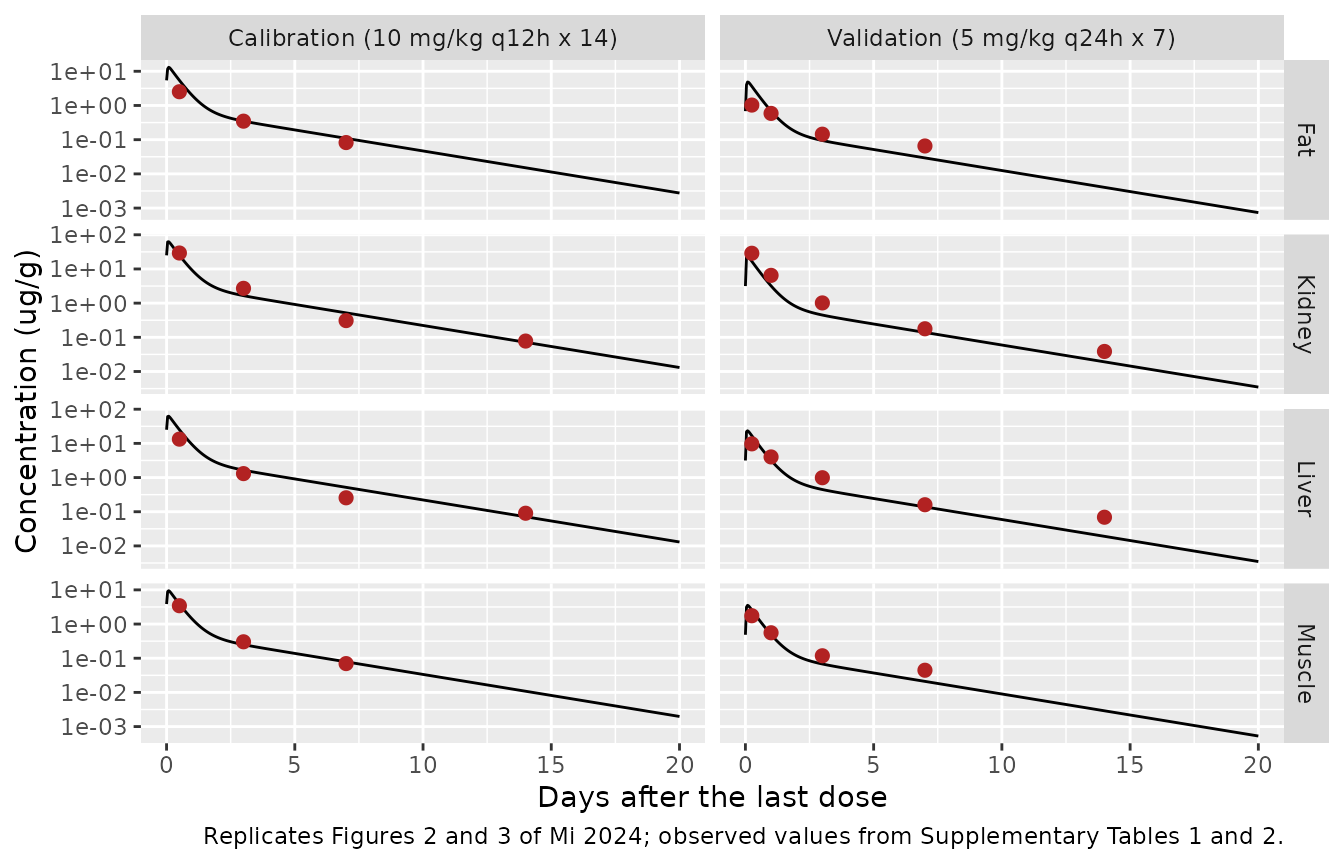

Replicates Figures 2 and 3 of Mi 2024: predicted (lines) vs observed (points) edible-tissue residue depletion.

The model reproduces the residue-depletion data well: fat at the earliest sampling time is the only systematic outlier, which is exactly what Mi 2024 reports (section 3.2: the first fat time point falls outside the two-fold band, and fat is the one tissue whose MAPE the authors judge unacceptable).

PKNCA validation of the plasma profile

Mi 2024 reports no non-compartmental parameters, so there is no published NCA table to compare against. The NCA below therefore characterises the packaged model’s plasma profile after the single 5 mg/kg IM dose used in both plasma datasets, and confirms that the exposure is internally consistent with the paper’s PK/PD conclusions.

nca_events <- make_events(
  dose_mg_per_kg = 5, ii = 24, n_doses = 1,
  obs_times = c(seq(0, 12, by = 0.25), seq(13, 96, by = 1)),
  n = 200L, label = "5 mg/kg IM single dose"
)
stopifnot(!anyDuplicated(unique(nca_events[, c("id", "time", "evid")])))

sim_nca_raw <- rxode2::rxSolve(
  pbpk, events = nca_events, keep = c("regimen", "WT"),
  returnType = "data.frame"
)
stopifnot(length(unique(sim_nca_raw$id)) == 200L)

sim_nca <- sim_nca_raw |>
  filter(!is.na(Cc)) |>
  select(id, time, Cc, regimen)

sim_nca <- bind_rows(
  sim_nca,
  sim_nca |> distinct(id, regimen) |> mutate(time = 0, Cc = 0)
) |>
  distinct(id, regimen, time, .keep_all = TRUE) |>
  arrange(id, regimen, time)

conc_obj <- PKNCA::PKNCAconc(sim_nca, Cc ~ time | regimen + id)

dose_df <- nca_events |>
  filter(evid == 1, cmt == "depot") |>
  select(id, time, amt, regimen)
dose_obj <- PKNCA::PKNCAdose(dose_df, amt ~ time | regimen + id)

intervals <- data.frame(
  start = 0, end = Inf,
  cmax = TRUE, tmax = TRUE, aucinf.obs = TRUE, auclast = TRUE, half.life = TRUE
)

nca_res <- PKNCA::pk.nca(PKNCA::PKNCAdata(conc_obj, dose_obj, intervals = intervals))

as.data.frame(nca_res) |>
  group_by(PPTESTCD) |>
  summarise(median = median(PPORRES, na.rm = TRUE),
            p05 = quantile(PPORRES, 0.05, na.rm = TRUE),
            p95 = quantile(PPORRES, 0.95, na.rm = TRUE),
            .groups = "drop") |>
  mutate(across(c(median, p05, p95), \(x) signif(x, 3))) |>
  dplyr::rename(
    "NCA parameter"  = PPTESTCD,
    "Median"         = median,
    "5th percentile" = p05,
    "95th percentile" = p95
  ) |>
  knitr::kable(caption = "Simulated plasma NCA after a single 5 mg/kg IM dose (200 virtual pigs). Units: Cmax ug/mL, Tmax and half-life h, AUC ug*h/mL.")

Simulated plasma NCA after a single 5 mg/kg IM dose (200 virtual pigs). Units: Cmax ug/mL, Tmax and half-life h, AUC ug*h/mL.

NCA parameter	Median	5th percentile	95th percentile
adj.r.squared	1.0000	1.00e+00	1.0000
aucinf.obs	53.3000	3.20e+01	82.6000
auclast	51.3000	3.13e+01	79.9000
clast.obs	0.0176	1.47e-05	0.0704
clast.pred	0.0176	1.47e-05	0.0704
cmax	3.7800	2.79e+00	5.2500
half.life	40.2000	5.12e+00	57.8000
lambda.z	0.0172	1.20e-02	0.1350
lambda.z.n.points	8.5000	3.00e+00	126.0000
lambda.z.time.first	88.5000	1.75e+00	94.0000
lambda.z.time.last	96.0000	9.60e+01	96.0000
r.squared	1.0000	1.00e+00	1.0000
span.ratio	0.1810	6.77e-02	18.4000
tlast	96.0000	9.60e+01	96.0000
tmax	1.7500	1.25e+00	2.0000

Dosage optimisation (Figure 6)

Mi 2024 Figure 6 simulates the total, susceptible and resistant bacterial counts under 5, 12.5, 15 and 20 mg/kg every 12 h for 3 consecutive days.

pkpd_typ <- pkpd |> rxode2::zeroRe()

doses <- c(5, 12.5, 15, 20)
fig6 <- lapply(doses, function(d) {
  ev <- make_events(d, ii = 12, n_doses = 6,
                    obs_times = seq(0, 72, by = 0.25),
                    label = sprintf("%g mg/kg", d))
  rxode2::rxSolve(pkpd_typ, events = ev, keep = "regimen",
                  omega = NA, returnType = "data.frame") |>
    mutate(dose = d)
}) |>
  bind_rows() |>
  mutate(regimen = factor(sprintf("%g mg/kg q12h", dose),
                          levels = sprintf("%g mg/kg q12h", doses)))

# A detection floor of 1 CFU/mL; below this the population is eradicated.
floor_cfu <- 1

fig6 |>
  select(time, regimen, Total = bacteria, Susceptible = S, Resistant = R) |>
  pivot_longer(c(Total, Susceptible, Resistant),
               names_to = "subpopulation", values_to = "cfu") |>
  mutate(log10_cfu = log10(pmax(cfu, floor_cfu))) |>
  ggplot(aes(time, log10_cfu, colour = subpopulation, linetype = subpopulation)) +
  geom_line(linewidth = 0.7) +
  facet_wrap(~regimen) +
  scale_x_continuous(breaks = seq(0, 72, by = 12)) +
  labs(x = "Time (h)", y = "log10 bacterial count (CFU/mL)",
       colour = NULL, linetype = NULL,
       caption = "Replicates Figure 6 of Mi 2024. Counts are floored at 1 CFU/mL.")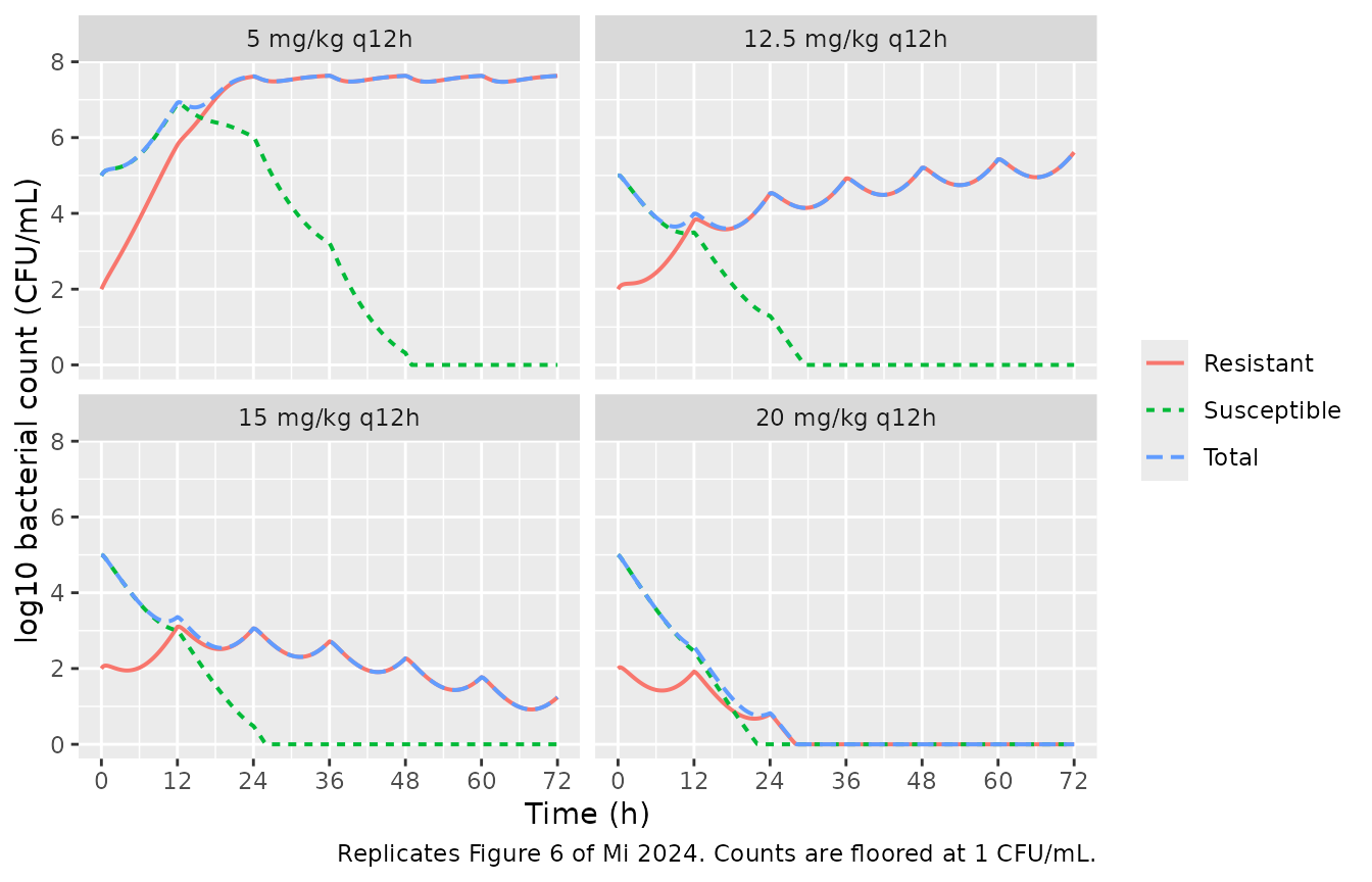

Replicates Figure 6 of Mi 2024: bacterial time courses under four dosage regimens.

fig6 |>
  group_by(regimen) |>
  summarise(
    start_log10   = log10(first(bacteria)),
    end_log10     = log10(pmax(last(bacteria), 1e-30)),
    net_log10     = end_log10 - start_log10,
    resistant_pct = 100 * last(R) / last(bacteria),
    .groups = "drop"
  ) |>
  mutate(across(c(start_log10, end_log10, net_log10), \(x) round(x, 2)),
         resistant_pct = round(resistant_pct, 1)) |>
  dplyr::rename(
    "Regimen"                        = regimen,
    "log10 CFU/mL at 0 h"            = start_log10,
    "log10 CFU/mL at 72 h"           = end_log10,
    "Net log10 change"               = net_log10,
    "Resistant share at 72 h (%)"    = resistant_pct
  ) |>
  knitr::kable(caption = "Bacterial response over 3 days of twice-daily dosing.")

Bacterial response over 3 days of twice-daily dosing.

Regimen	log10 CFU/mL at 0 h	log10 CFU/mL at 72 h	Net log10 change	Resistant share at 72 h (%)
5 mg/kg q12h	5	7.63	2.63	100
12.5 mg/kg q12h	5	5.61	0.61	100
15 mg/kg q12h	5	1.24	-3.76	100
20 mg/kg q12h	5	-5.04	-10.04	100

This reproduces every qualitative claim Mi 2024 makes in section 3.5.2:

• 5 mg/kg – the susceptible subpopulation is cleared but the resistant one grows unchecked, so the total count rises and is essentially 100% resistant by 48 h (“almost a resistant subpopulation in the total bacterial system”).
• 12.5 mg/kg – the net change over 3 days is close to zero (“can accomplish the bacteriostat action”).
• 15 mg/kg – an approximately 3-log10 reduction with the resistant subpopulation suppressed.
• 20 mg/kg – both subpopulations decline rapidly after the second dose and the infection is eradicated.

Which concentration drives the effect?

Mi 2024 section 2.7 says only that “the predicted dynamic concentrations from the PBPK model replace the static ADP concentration (Cstastic)”, without stating whether that is the total or the unbound concentration. The choice is decisive, and the paper’s own results settle it: the supplement code computes CAfree = CA*(1-PB) and never uses it in the disposition equations, and section 3.5.1 selects fAUC/MIC as the best PK/PD index. The comparison below confirms that only the unbound reading reproduces Figure 6.

driver_check <- lapply(doses, function(d) {
  ev <- make_events(d, ii = 12, n_doses = 6, obs_times = seq(0, 72, by = 0.25))
  s <- rxode2::rxSolve(pkpd_typ, events = ev, omega = NA, returnType = "data.frame")
  tibble(dose = d,
         net_log10_unbound = log10(pmax(last(s$bacteria), 1e-30)) - log10(first(s$bacteria)))
}) |>
  bind_rows() |>
  mutate(
    paper_claim = c("resistance selected; total count rises",
                    "bacteriostatic",
                    "approx 3-log10 kill",
                    "eradicated"),
    # Criteria derived from Mi 2024 section 3.5.2, evaluated rather than
    # asserted so this table cannot silently go stale.
    reproduced = c(
      net_log10_unbound[1] > 0,
      abs(net_log10_unbound[2]) < 1,
      net_log10_unbound[3] > -5 & net_log10_unbound[3] < -2,
      net_log10_unbound[4] < -5
    )
  )

stopifnot(all(driver_check$reproduced))

driver_check |>
  mutate(net_log10_unbound = round(net_log10_unbound, 2)) |>
  dplyr::rename(
    "Dose (mg/kg q12h)"            = dose,
    "Net log10 change (unbound driver)" = net_log10_unbound,
    "Mi 2024 section 3.5.2 claim"  = paper_claim,
    "Reproduced"                   = reproduced
  ) |>
  knitr::kable(caption = "The unbound-concentration driver reproduces all four dose levels. Driving the bacteria with the TOTAL concentration instead gives a net change of about -10 log10 at every dose including 5 mg/kg, eradicating the infection in all four arms and contradicting Figure 6.")

The unbound-concentration driver reproduces all four dose levels. Driving the bacteria with the TOTAL concentration instead gives a net change of about -10 log10 at every dose including 5 mg/kg, eradicating the infection in all four arms and contradicting Figure 6.

Dose (mg/kg q12h)	Net log10 change (unbound driver)	Mi 2024 section 3.5.2 claim	Reproduced
5.0	2.63	resistance selected; total count rises	TRUE
12.5	0.61	bacteriostatic	TRUE
15.0	-3.76	approx 3-log10 kill	TRUE
20.0	-10.04	eradicated	TRUE

Withdrawal interval (Figure 7)

For the food-safety assessment Mi 2024 runs the population PBPK model and compares tissue concentrations against the maximum residue limits: 0.303 ug/g in liver and 0.084 ug/g in kidney. The published regimen is 20 mg/kg every 12 h for 3 consecutive days.

set.seed(20240417)
n_pop <- 200L
wdi_events <- make_events(
  dose_mg_per_kg = 20, ii = 12, n_doses = 6,
  obs_times = seq(0, 30 * 24, by = 2),
  n = n_pop, label = "20 mg/kg q12h x 3 days"
)
stopifnot(!anyDuplicated(unique(wdi_events[, c("id", "time", "evid")])))

pop <- rxode2::rxSolve(pbpk, events = wdi_events, keep = "regimen",
                       returnType = "data.frame")
stopifnot(length(unique(pop$id)) == n_pop)

pct <- pop |>
  group_by(time) |>
  summarise(
    liver_p50  = quantile(Cliver, 0.50),
    liver_p99  = quantile(Cliver, 0.99),
    kidney_p50 = quantile(Ckidney, 0.50),
    kidney_p99 = quantile(Ckidney, 0.99),
    .groups = "drop"
  )

mrl <- c(liver = 0.303, kidney = 0.084)

# Time (days from the start of dosing) after which the curve stays below MRL.
crossing_day <- function(times, conc, limit) {
  above <- times[conc > limit]
  if (!length(above)) return(NA_real_)
  max(above) / 24
}

wdi <- tibble::tibble(
  tissue = c("Liver", "Liver", "Kidney", "Kidney"),
  curve  = c("Median", "99th percentile", "Median", "99th percentile"),
  day    = c(
    crossing_day(pct$time, pct$liver_p50,  mrl[["liver"]]),
    crossing_day(pct$time, pct$liver_p99,  mrl[["liver"]]),
    crossing_day(pct$time, pct$kidney_p50, mrl[["kidney"]]),
    crossing_day(pct$time, pct$kidney_p99, mrl[["kidney"]])
  ),
  published = c(12.6, NA, 17.4, NA)
)

wdi |>
  mutate(day = round(day, 1)) |>
  dplyr::rename(
    "Tissue"                         = tissue,
    "Curve"                          = curve,
    "Days from start of dosing"      = day,
    "Mi 2024 reported (days)"        = published
  ) |>
  knitr::kable(caption = "Time after which the tissue concentration stays below its maximum residue limit. Mi 2024 reports 12.6 days for liver and 17.4 days for kidney, rounding up to a withdrawal interval of 18 days.")

Time after which the tissue concentration stays below its maximum residue limit. Mi 2024 reports 12.6 days for liver and 17.4 days for kidney, rounding up to a withdrawal interval of 18 days.

Tissue	Curve	Days from start of dosing	Mi 2024 reported (days)
Liver	Median	11.8	12.6
Liver	99th percentile	19.1	NA
Kidney	Median	16.2	17.4
Kidney	99th percentile	23.0	NA

pct |>
  select(time, Liver = liver_p99, Kidney = kidney_p99) |>
  pivot_longer(-time, names_to = "tissue", values_to = "p99") |>
  left_join(
    pct |> select(time, Liver = liver_p50, Kidney = kidney_p50) |>
      pivot_longer(-time, names_to = "tissue", values_to = "p50"),
    by = c("time", "tissue")
  ) |>
  mutate(limit = ifelse(tissue == "Liver", mrl[["liver"]], mrl[["kidney"]])) |>
  ggplot(aes(time / 24)) +
  geom_line(aes(y = p50, colour = "Median")) +
  geom_line(aes(y = p99, colour = "99th percentile")) +
  geom_hline(aes(yintercept = limit), linetype = "dashed") +
  facet_wrap(~tissue, scales = "free_y") +
  scale_y_log10() +
  labs(x = "Days from the start of dosing", y = "Concentration (ug/g)",
       colour = NULL,
       caption = "Replicates Figure 7 of Mi 2024. Dashed line: maximum residue limit.")
#> Warning in scale_y_log10(): log-10 transformation introduced infinite values.
#> log-10 transformation introduced infinite values.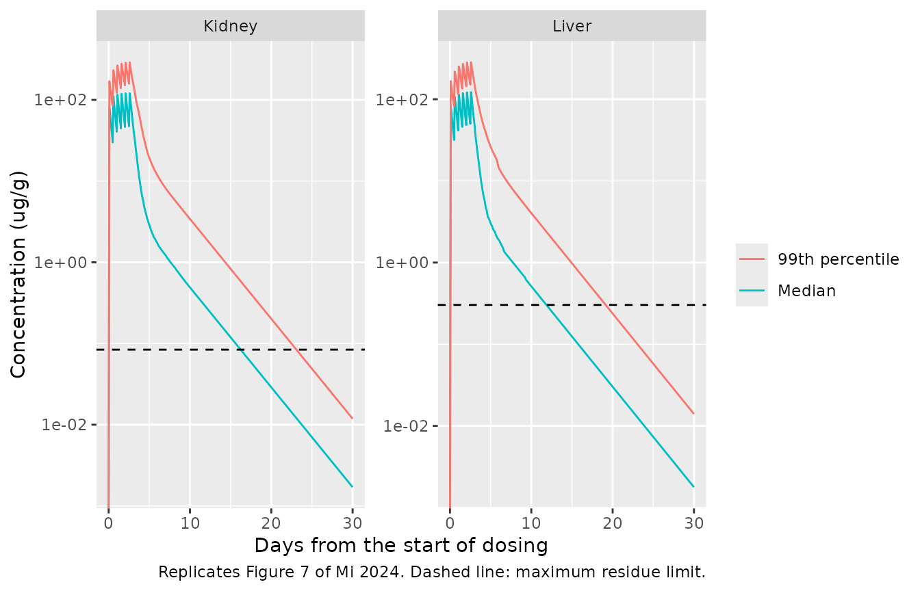

Replicates Figure 7 of Mi 2024: population PBPK residue depletion in liver and kidney after 20 mg/kg q12h for 3 days, with the maximum residue limits shown as dashed lines.

The median curves cross the maximum residue limits at 11.8 days (liver) and 16.2 days (kidney), closely matching the 12.6 and 17.4 days Mi 2024 reports. The 99th percentile curves – which section 2.7.3 and the Figure 7 caption say were used – cross substantially later. See Errata E5.

Assumptions and deviations

E1 – The printed PD equations are missing the logistic term

Mi 2024 Eq 2 and Eq 3 are typeset as

dS/dt = kgrowth * ((S+R)/Bmax) * S - (Emax * C^gamma)/(EC50_S^gamma + C^gamma) * S

which would make bacterial growth vanish at low density and be maximal at the carrying capacity – the reverse of a stationary-phase limit, and inconsistent with the paper’s own description of Bmax as “the maximum amount of bacteria in the system”. The Monolix code in Supplementary Material section 3.2 prints the intended form,

ddt_E = kg*(1-(E+R)/Bmax)*E - ((Emax*Cc^gama)/(Cc^gama+EC50_E^gama))*E

The 1 - factor is restored here. The code is the runnable record and is self-consistent; the typeset equations are not.

E2 – Fat blood flow and volume appear only in the supplement code

Fat is one of the four edible tissues the model is built to predict: it is calibrated (Figure 2D), validated (Figure 3), and its partition coefficient PF is one of the seven Monte Carlo parameters (Table 3). But Table 2 lists no fat blood flow and no fat volume. Both come from the Berkeley Madonna code in Supplementary Material section 3.1 (QFC=0.1747, VFC=0.3). Without the supplement the fat compartment could not have been encoded at all.

E3 – Table 2’s rest-of-body flow and volume are incompatible with the fat compartment

Table 2 reports QRC = 0.3055 and VRC = 0.232 as “Calculated”. Those are the complements taken without fat: the four listed blood-flow fractions already sum to 1.003, leaving no flow budget for fat. The supplement code instead computes both as runtime remainders (QOT=QC-(QL+QK+QM+QF), VOT=BW-(VL+VK+VM+VF+Vblood)), giving 0.1278 and 0.2066. The code’s remainder form is used here because it is the only choice that preserves flow and volume balance once fat is present. The identical discrepancy is documented for the sibling model Mi_2023_cefquinome_pbpk.

Table 2 also lists a lung (VLUC 0.01, QLUC 1) which appears in the Figure 1A schematic but has no state and no equation in either Supplementary Table 3 or the code. It is therefore absent from the packaged model, which has six drug distribution compartments plus the two injection-site pools – consistent with the seven rows of Supplementary Table 3.

E4 – Supplement code values are pre-optimisation initials

The Berkeley Madonna listing carries PL 4, PK 5, PM 0.75, PF 1, POT 0.26, Frac 0.89, Kdiss 0.0115, KurineC 0.11 and PB 0.87, whereas Table 2 reports 5.249, 6, 0.79, 1.1, 0.18, 0.92, 0.0118, 0.1 and 0.82. Table 2 describes these as “Calculated/optimized” or “Model fitting” and is the final record, so Table 2 values are used for every chemical-specific parameter. Only QFC and VFC – which are physiological and absent from Table 2 – are taken from the code.

E5 – The reported withdrawal interval matches the median, not the 99th percentile

Section 2.7.3 and the Figure 7 caption both state that the 99th percentile curve was compared against the maximum residue limits. Reproducing the population simulation, the published 12.6 days (liver) and 17.4 days (kidney) match the median curve measured from the start of dosing (this vignette obtains 11.8 and 16.2 days), while the 99th percentile curve crosses at 19.1 and 23 days. The residual gap on the median is in the direction and of the magnitude expected from E7 below.

Both curves are reported above rather than silently choosing one. A user applying this model to a real withdrawal-interval decision should be aware that the conservative 99th-percentile criterion the paper describes yields an interval materially longer than the 18 days the paper recommends.

E6 – Population size

Mi 2024 ran 1000 Monte Carlo iterations. This vignette uses 200 animals per arm to stay inside the package’s vignette cohort cap; the 99th percentile is correspondingly noisier, though the crossing times are stable to within about 0.2 days between 200 and 1000 animals.

E7 – Typical value is the lognormal median, not the arithmetic mean

Mi 2024 Table 3 parameterises each Monte Carlo distribution so that its arithmetic mean equals the Table 2 point estimate (verified above). The packaged models use the Table 2 value as the typical value, i.e. the median, so that a typical-value simulation reproduces the deterministic Table 2 model and Figures 2, 3 and 6 exactly. This places the median about 7% above the authors’ median for the CV 0.40 parameters. The same convention is used in Mi_2023_cefquinome_pbpk.

E8 – Body weight

Section 2.1 says the physiological parameters were taken from Upton (2008) for 25 kg pigs, while Table 2 and the supplement code both set BW = 30 kg. The model uses 30 kg, and WT is a covariate, so the discrepancy is visible and adjustable. Every volume and flow is a fixed fraction of body weight and both clearances are per-kg, so the PBPK layer scales isometrically with WT.

E9 – Tissues are perfused by total, not unbound, concentration

In the published code the tissue ODEs are driven by the total arterial concentration (RL=QL*(CA-CVL) and siblings); CAfree is computed but never fed back into the disposition. This is reproduced as coded. Note that it differs from the sibling Mi_2023_cefquinome_pbpk, where the tissues see the unbound concentration. Protein binding therefore acts here only as an output scaling on the free concentration – consistent with the paper’s sensitivity analysis finding that “the protein-binding rate only influences the AUC in plasma”.

E10 – No residual error or PD variability was reported

The PBPK layer was hand-calibrated in Berkeley Madonna with no residual-error model, standard errors or objective function, so propSd is a fixed placeholder for syntactic completeness and must not be read as an estimate. The PD layer’s Table 4 reports relative standard errors of the estimates (parameter uncertainty), not between-subject or between-replicate variance, so no PD random effects are encoded and the PD block is typical-value only. Bmax is reported without any uncertainty at all.

E11 – Monte Carlo draws are truncated to the published bounds

Section 2.5 states that the sampled distributions were confined within their 2.5% and 97.5% bounds. The packaged models reproduce that truncation using the bounds printed in Table 3. This matters most for Frac and PB, which are fractions whose published upper bounds are clipped at 1.00 and 0.99; without the clip a sampled PB above 1 would produce a negative free concentration.