Artemether + lumefantrine PK + parasitemia PD (Hietala 2010)
Source:vignettes/articles/Hietala_2010_artemether_lumefantrine_malaria.Rmd
Hietala_2010_artemether_lumefantrine_malaria.RmdModel and source
- Citation: Friberg Hietala S, Martensson A, Ngasala B, Dahlstrom S, Lindegardh N, Annerberg A, Premji Z, Farnert A, Gil P, Bjorkman A, Ashton M (2010). Population pharmacokinetics and pharmacodynamics of artemether and lumefantrine during combination treatment in children with uncomplicated falciparum malaria in Tanzania. Antimicrob Agents Chemother 54(11):4780-4788.
- Article: https://doi.org/10.1128/AAC.00252-10
- ClinicalTrials.gov: NCT00336375
Hietala 2010 reports three coupled models from a single Coartem pediatric trial in Tanzania:
- a joint two-compartment artemether (ARM) + one-compartment dihydroartemisinin (DHA) PK model with time-dependent ARM clearance across the six-dose regimen (Table 1),
- a one-compartment lumefantrine (LUM) PK model with absorption lag (Table 2), and
- a five-stage semi-mechanistic parasite-dynamics PD model driven by the ARM/DHA exposures (Table 3).
Per the replicate-author-structure policy each fit is
extracted as its own model file, with this single vignette walking the
paper as a unit:
mod_arm_fn          <- readModelDb("Hietala_2010_artemether")
mod_lum_fn          <- readModelDb("Hietala_2010_lumefantrine")
mod_pd_fn           <- readModelDb("Hietala_2010_artemether_parasitemia")

mod_arm <- rxode2::rxode2(mod_arm_fn())
mod_lum <- rxode2::rxode2(mod_lum_fn())
mod_pd  <- rxode2::rxode2(mod_pd_fn())
Population
Hietala 2010 enrolled 50 Tanzanian children (19 male, 31 female; ages
1-10 years, mean 4; weights 8-30 kg, mean 14) with acute uncomplicated
Plasmodium falciparum malaria (admission parasite densities
2,000-200,000 / microL with fever, or history of fever within 24 h). All
received the standard six-dose weight-based Coartem regimen (20 mg
artemether + 120 mg lumefantrine per tablet; 1-3 tablets per dose based
on weight band) at 0, 8, 24, 36, 48, and 60 h, half randomised to take
each dose with 200 mL of full-fat (3.4%) cow’s milk and half with water
(milk completion 43% of intended dose occasions). The parasite-dynamics
arm additionally drew 104 capillary parasite counts from 11 asymptomatic
children from the same coastal region for the steady-state asymptomatic
parameterisation (REPL_a = 1, A_a = 1.01; not encoded in
Hietala_2010_artemether_parasitemia, see Assumptions).
Demographics summary from Results / Materials and Methods; programmatic
equivalents are available via
readModelDb("<...>")$population.
Source trace
Per-parameter source locations are recorded inline in each
inst/modeldb/specificDrugs/Hietala_2010_*.R next to the
ini() entry. The tables below collect them in one place for
review.
ARM / DHA PK (Hietala_2010_artemether and the embedded PK in Hietala_2010_artemether_parasitemia)
| Equation / parameter | Value | Source location |
|---|---|---|
lka <- fixed(log(1)) (ka, 1/h) |
1 (fixed) | Table 1 |
lcl <- log(2.6) (CL/F_ARM at OCC = 1, L/h/kg) |
2.6 | Table 1 (95% CI 1.5-2.6) |
e_occ_cl <- 0.57 (fractional CL/F_ARM increase per
OCC step) |
0.57 | Table 1 (95% CI 0.39-0.75) |
lvc <- log(5.2) (Vc/F_ARM, L/kg) |
5.2 | Table 1 (95% CI 3.5-7.1) |
lq <- log(1.4) (Q/F_ARM, L/h/kg) |
1.4 | Table 1 (95% CI 1.1-1.8) |
lvp <- log(41.4) (Vp/F_ARM, L/kg) |
41.4 | Table 1 (95% CI 29.0-58.1) |
lcl_dihydroart <- log(6.8) (CL/F_DHA, L/h/kg; F_DHA
fixed to 1) |
6.8 | Table 1 (95% CI 5.8-8.0) |
lvc_dihydroart <- log(3.7) (V/F_DHA, L/kg) |
3.7 | Table 1 (95% CI 2.3-8.7) |
etalcl ~ 0.155649 (CL/F_ARM IIV) |
CV 41% | Table 1 (95% CI 37-50) -> omega^2 = log(0.41^2 + 1) |
etalcl_dihydroart ~ 0.198101 (CL/F_DHA IIV) |
CV 47% | Table 1 (95% CI 35-57) -> omega^2 = log(0.47^2 + 1) |
propSd <- 0.61, addSd <- fixed(2)
(ARM residual) |
61% prop, 2 nM add (fixed) | Table 1 |
propSd_dihydroart <- 0.82,
addSd_dihydroart <- fixed(3) (DHA residual) |
82% prop, 3 nM add (fixed) | Table 1 |
| 2-cmt ARM with first-order absorption; 1-cmt DHA via complete 1:1 molar conversion | – | Results ‘Pharmacokinetics of artemether, dihydroartemisinin, and lumefantrine’; mass factor MW_DHA / MW_ARM = 284.3 / 298.4 |
| CL/F_ARM = theta1 * (1 + theta2 * (OCC - 1)) * exp(eta) | – | Results paragraph after Table 1 (delta-OFV = -167) |
LUM PK (Hietala_2010_lumefantrine)
| Equation / parameter | Value | Source location |
|---|---|---|
ltlag <- log(1.92) (absorption lag, h) |
1.92 | Table 2 (95% CI 1.86-1.96) |
lka <- log(0.82) (ka, 1/h) |
0.82 | Table 2 (95% CI 0.45-1.61) |
lcl <- log(0.077) (CL/F, L/h/kg = 77 mL/h/kg) |
77 mL/h/kg | Table 2 (95% CI 52-105 mL/h/kg) |
lvc <- log(8.9) (V/F, L/kg) |
8.9 | Table 2 (95% CI 6.8-11.7) |
etalka ~ 1.241237 (ka IIV) |
CV 156% | Table 2 (95% CI 126-190) -> omega^2 = log(1.56^2 + 1) |
etalvc ~ 0.515660 (V/F IIV) |
CV 82% | Table 2 (95% CI 66-102) -> omega^2 = log(0.82^2 + 1) |
propSd <- 0.46, addSd <- 43 (LUM
residual) |
46% prop, 43 nM add | Table 2 |
| 1-cmt with absorption lag | – | Results ‘PK of LUM was best described by a one-compartment model with a combined proportional and additive residual error. The introduction of an absorption lag time significantly improved the model (delta-OFV = -96).’ |
| Milk intake covariate not retained | – | Results ‘The inclusion of milk intake as a covariate … did not result in an improvement of the model.’ |
Parasite PD (Hietala_2010_artemether_parasitemia, symptomatic-patient parameterisation)
| Equation / parameter | Value | Source location |
|---|---|---|
p_init <- fixed(1) (initial parasitemia,
parasites/microL) |
1 (fixed) | Table 3 |
etap_init ~ 1.005 (P_init IIV) |
CV 119.2% | Table 3 (95% CI 98-161) -> omega^2 = log(1.192^2 + 1) |
lvpt <- log(15.5) (VPT, h; visible-stage mean
transit time) |
15.5 | Table 3 (95% CI 9.7-21.5) |
lmtt <- log(48.5) (MTT, h; intraerythrocytic cycle
time) |
48.5 | Table 3 (95% CI 48.0-49.1) |
repl <- 4 (REPL_p) |
4 | Table 3 (95% CI 3.6-4.4); ‘~12-fold per cycle’ Discussion |
amp <- fixed(0) (A_p) |
0 (fixed) | Table 3 (sine modulation absent in symptomatic patients) |
lkspleen <- fixed(log(0.26)) (k_spleen, 1/h) |
0.26 (fixed) | Table 3 (ref 9, Gordi 2005) |
s_armdha <- 0.073 (shared ARM/DHA log-conc kill
slope) |
0.073 | Table 3 (95% CI 0.049-0.423) |
propSd_visibleParasitemia <- 1.38 (residual
sigma) |
138% | Table 3 (95% CI 125-258); proportional on log-transformed parasitemia |
| k_VPT = 3 / VPT (visible-stage transition rate) | – | Results ‘mean rate of transfer between visible compartments, k_VPT, was modeled as 3/VPT’ |
| k_IPT = 1 / (MTT - VPT) (sequestered-to-PTR rate) | – | Results ‘mean time for transfer from the sequestered state, k_IPT, was fixed to 1/(MTT - VPT)’ |
| k_ARM = S_ARMDHA * log[ARM]; k_DHA = S_ARMDHA * log[DHA] | – | Results ‘The effects of ARM and DHA plasma concentrations were modeled on all developmental stages as …’ |
| Visible parasitemia = PTR + PSR + PLR + Pspleen | – | Methods ‘Only the parasites in the ring stages and those injured by drugs were assumed to be visible through microscopy.’ |
| Infection started 4 cycles (= 4 * MTT) before first sample | – | Results ‘The number of cycles passed since model initiation was fixed to 4 in patients.’ |
Virtual cohort
Body-weight distribution approximates the Tanzanian pediatric cohort (mean 14 kg, range 8-30 kg). Both PK models (ARM/DHA and LUM) use linear (per-kg) weight normalisation; the PD model carries the same per-kg PK structure plus a single body-weight covariate.
set.seed(20260601L)
n_sub <- 40L

subjects <- data.frame(
  id        = seq_len(n_sub),
  WT        = round(pmin(pmax(rnorm(n_sub, mean = 14, sd = 4.5), 8), 30), 1),
  treatment = "Coartem (6 doses)"
)
Dose schedule from Materials and Methods: six oral doses at 0, 8, 24, 36, 48, and 60 hours. Tablet count is weight-banded (5-14 kg -> 1 tablet, 15-24 kg -> 2 tablets, 25-34 kg -> 3 tablets); each tablet is 20 mg ARM + 120 mg LUM.
dose_times <- c(0, 8, 24, 36, 48, 60)

tablet_count <- function(wt) {
  ifelse(wt <= 14, 1L,
         ifelse(wt <= 24, 2L, 3L))
}

# Observation grid: dense over the dosing window so peak / trough features
# resolve, sparse-but-regular over the 60-72 h post-last-dose tail. Kept
# coarse (every 1 h) to keep the vignette under the 5-minute render budget.
obs_times <- sort(unique(c(
  seq(0, 60, by = 1),
  seq(60.5, 72, by = 0.5)
)))

# OCC indicator: dose number 1..6 at each time point, propagating from the
# most recent dose. Used to drive CL/F_ARM(OCC) = theta1 * (1 + theta2 * (OCC
# - 1)) inside model().
occ_at <- function(t) {
  occ <- findInterval(t, dose_times) # gives 1..6 for t in [0,8), [8,24), ...
  pmin(pmax(occ, 1L), length(dose_times))
}
ARM / DHA PK simulation
build_arm_events <- function(subjects, obs_times, dose_times) {
  out <- vector("list", length = nrow(subjects))
  for (i in seq_len(nrow(subjects))) {
    s <- subjects[i, ]
    arm_per_tab_mg <- 20
    dose_amt <- arm_per_tab_mg * tablet_count(s$WT)
    dose_rows <- data.frame(
      id        = s$id,
      time      = dose_times,
      evid      = 1L,
      amt       = dose_amt,
      cmt       = "depot",
      WT        = s$WT,
      OCC       = seq_along(dose_times),
      treatment = s$treatment
    )
    obs_rows <- data.frame(
      id        = s$id,
      time      = obs_times,
      evid      = 0L,
      amt       = 0,
      cmt       = "Cc",
      WT        = s$WT,
      OCC       = occ_at(obs_times),
      treatment = s$treatment
    )
    out[[i]] <- rbind(dose_rows, obs_rows)
  }
  events <- dplyr::bind_rows(out)
  events[order(events$id, events$time, -events$evid), ]
}

events_arm <- build_arm_events(subjects, obs_times, dose_times)
stopifnot(!anyDuplicated(unique(events_arm[, c("id", "time", "evid", "cmt")])))

sim_arm <- rxode2::rxSolve(
  mod_arm,
  events = events_arm,
  keep   = c("WT", "OCC", "treatment")
) |>
  as.data.frame()
Median (5th-95th simulated percentile) ARM and DHA plasma concentrations over 0-72 h:
sim_long <- sim_arm |>
  dplyr::filter(!is.na(Cc)) |>
  dplyr::select(id, time, Cc, Cc_dihydroart) |>
  tidyr::pivot_longer(c(Cc, Cc_dihydroart), names_to = "analyte", values_to = "value") |>
  dplyr::mutate(analyte = dplyr::recode(analyte, Cc = "Artemether", Cc_dihydroart = "DHA"))

sim_long |>
  dplyr::group_by(analyte, time) |>
  dplyr::summarise(
    p05 = quantile(value, 0.05, na.rm = TRUE),
    p50 = quantile(value, 0.50, na.rm = TRUE),
    p95 = quantile(value, 0.95, na.rm = TRUE),
    .groups = "drop"
  ) |>
  dplyr::filter(p50 > 0) |>
  ggplot(aes(time, p50, colour = analyte, fill = analyte)) +
  geom_ribbon(aes(ymin = p05, ymax = p95), alpha = 0.20, colour = NA) +
  geom_line(linewidth = 0.6) +
  scale_y_log10() +
  labs(x = "Time (hours)",
       y = "Plasma concentration (nM)",
       title = "ARM and DHA plasma concentrations over the six-dose Coartem regimen",
       caption = "Replicates the shape of Figure 1 of Hietala 2010 (ARM solid, DHA dashed in the original).")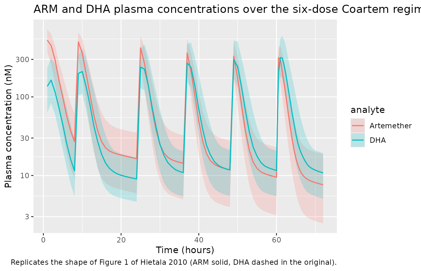
The time-dependent CL/F_ARM produces visibly lower trough concentrations at later doses, matching the trend in Figure 4 of the source paper (~3.4-fold increase in CL/F_ARM between dose 1 and dose 6).
LUM PK simulation
build_lum_events <- function(subjects, obs_times, dose_times) {
  out <- vector("list", length = nrow(subjects))
  for (i in seq_len(nrow(subjects))) {
    s <- subjects[i, ]
    lum_per_tab_mg <- 120
    dose_amt <- lum_per_tab_mg * tablet_count(s$WT)
    dose_rows <- data.frame(
      id        = s$id,
      time      = dose_times,
      evid      = 1L,
      amt       = dose_amt,
      cmt       = "depot",
      WT        = s$WT,
      treatment = s$treatment
    )
    obs_rows <- data.frame(
      id        = s$id,
      time      = obs_times,
      evid      = 0L,
      amt       = 0,
      cmt       = "Cc",
      WT        = s$WT,
      treatment = s$treatment
    )
    out[[i]] <- rbind(dose_rows, obs_rows)
  }
  events <- dplyr::bind_rows(out)
  events[order(events$id, events$time, -events$evid), ]
}

events_lum <- build_lum_events(subjects, obs_times, dose_times)
stopifnot(!anyDuplicated(unique(events_lum[, c("id", "time", "evid", "cmt")])))

sim_lum <- rxode2::rxSolve(
  mod_lum,
  events = events_lum,
  keep   = c("WT", "treatment")
) |>
  as.data.frame()
sim_lum |>
  dplyr::filter(!is.na(Cc)) |>
  dplyr::group_by(time) |>
  dplyr::summarise(
    p05 = quantile(Cc, 0.05, na.rm = TRUE),
    p50 = quantile(Cc, 0.50, na.rm = TRUE),
    p95 = quantile(Cc, 0.95, na.rm = TRUE),
    .groups = "drop"
  ) |>
  dplyr::filter(p50 > 0) |>
  ggplot(aes(time, p50)) +
  geom_ribbon(aes(ymin = p05, ymax = p95), alpha = 0.25) +
  geom_line(linewidth = 0.6) +
  labs(x = "Time (hours)",
       y = "Lumefantrine plasma concentration (nM)",
       title = "LUM plasma concentrations over the six-dose Coartem regimen",
       caption = "Replicates the shape of Figure 2 of Hietala 2010.")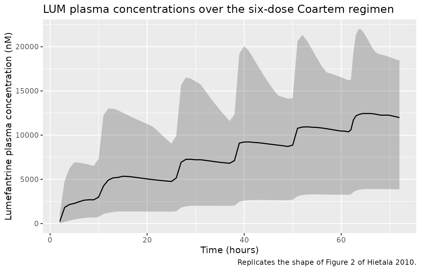
Hietala 2010 reports a typical-value LUM day-3 median plasma concentration of 9.3 microM (Discussion). Our typical-subject simulation:
mod_lum_typical    <- rxode2::zeroRe(mod_lum)
typical_subjects   <- data.frame(id = 1L, WT = 14, treatment = "Typical (WT = 14 kg)")
events_lum_typical <- build_lum_events(typical_subjects, obs_times, dose_times)
sim_lum_typical    <- rxode2::rxSolve(mod_lum_typical, events = events_lum_typical,
                                      keep = c("WT", "treatment")) |>
  as.data.frame()
#> ℹ omega/sigma items treated as zero: 'etalka', 'etalvc'

lum_day3_nM <- sim_lum_typical$Cc[sim_lum_typical$time == 72]
sprintf("Simulated typical-subject LUM at 72 h (day 3): %.2f microM (paper Discussion: 9.3 microM)",
        lum_day3_nM / 1000)
#> [1] "Simulated typical-subject LUM at 72 h (day 3): 7.89 microM (paper Discussion: 9.3 microM)"
Parasitemia PD simulation
The parasite life-cycle PD model is initiated by introducing
p_init parasites into the tinyrings compartment 4
intraerythrocytic cycles (4 * MTT = 194 h) before the first Coartem
dose, so the parasite population can grow to clinically realistic
admission parasitemia under the symptomatic-patient replication factor
REPL_p = 4 (Results, “The number of cycles passed since model initiation
was fixed to 4 in patients”). The timeline is therefore shifted so that
the first dose lands at simulation time 194 h, and observations span
0-266 h (= 194 + 72) of simulation time.
mtt          <- 48.5
n_pre_cycles <- 4
t_pre        <- n_pre_cycles * mtt           # 194 h
shift        <- t_pre

dose_times_pd <- shift + dose_times          # 194, 202, 218, 230, 242, 254
obs_times_pd  <- sort(unique(c(
  seq(0,             shift,      by = 12),
  seq(shift + 1,     shift + 60, by = 1),
  seq(shift + 60.5,  shift + 72, by = 0.5)
)))

build_pd_events <- function(subjects, obs_times_pd, dose_times_pd) {
  out <- vector("list", length = nrow(subjects))
  for (i in seq_len(nrow(subjects))) {
    s <- subjects[i, ]
    arm_per_tab_mg <- 20
    dose_amt <- arm_per_tab_mg * tablet_count(s$WT)
    dose_rows <- data.frame(
      id        = s$id,
      time      = dose_times_pd,
      evid      = 1L,
      amt       = dose_amt,
      cmt       = "depot",
      WT        = s$WT,
      OCC       = seq_along(dose_times_pd),
      treatment = s$treatment
    )
    obs_occ <- findInterval(obs_times_pd, dose_times_pd)
    obs_occ <- pmin(pmax(obs_occ, 1L), length(dose_times_pd))
    obs_rows <- data.frame(
      id        = s$id,
      time      = obs_times_pd,
      evid      = 0L,
      amt       = 0,
      cmt       = "visibleParasitemia",
      WT        = s$WT,
      OCC       = obs_occ,
      treatment = s$treatment
    )
    out[[i]] <- rbind(dose_rows, obs_rows)
  }
  events <- dplyr::bind_rows(out)
  events[order(events$id, events$time, -events$evid), ]
}

events_pd <- build_pd_events(subjects, obs_times_pd, dose_times_pd)
stopifnot(!anyDuplicated(unique(events_pd[, c("id", "time", "evid", "cmt")])))

sim_pd <- rxode2::rxSolve(
  mod_pd,
  events = events_pd,
  keep   = c("WT", "OCC", "treatment")
) |>
  as.data.frame()
sim_pd_vis <- sim_pd |>
  dplyr::filter(!is.na(visibleParasitemia), visibleParasitemia > 0) |>
  dplyr::mutate(time_post_dose = time - shift)

sim_pd_vis |>
  dplyr::group_by(time_post_dose) |>
  dplyr::summarise(
    p05 = quantile(visibleParasitemia, 0.05, na.rm = TRUE),
    p50 = quantile(visibleParasitemia, 0.50, na.rm = TRUE),
    p95 = quantile(visibleParasitemia, 0.95, na.rm = TRUE),
    .groups = "drop"
  ) |>
  dplyr::filter(p50 > 0) |>
  ggplot(aes(time_post_dose, p50)) +
  geom_ribbon(aes(ymin = pmax(p05, 1), ymax = p95), alpha = 0.25) +
  geom_line(linewidth = 0.6) +
  geom_vline(xintercept = 0, linetype = "dotted", colour = "grey50") +
  scale_y_log10() +
  labs(x = "Time relative to first Coartem dose (hours)",
       y = "Visible parasitemia (parasites / microL)",
       title = "Simulated parasite-density trajectory under Coartem treatment",
       caption = paste(
         "Negative times = pre-treatment growth from P_init.",
         "Replicates the shape of Figures 3 and 7 of Hietala 2010."
       ))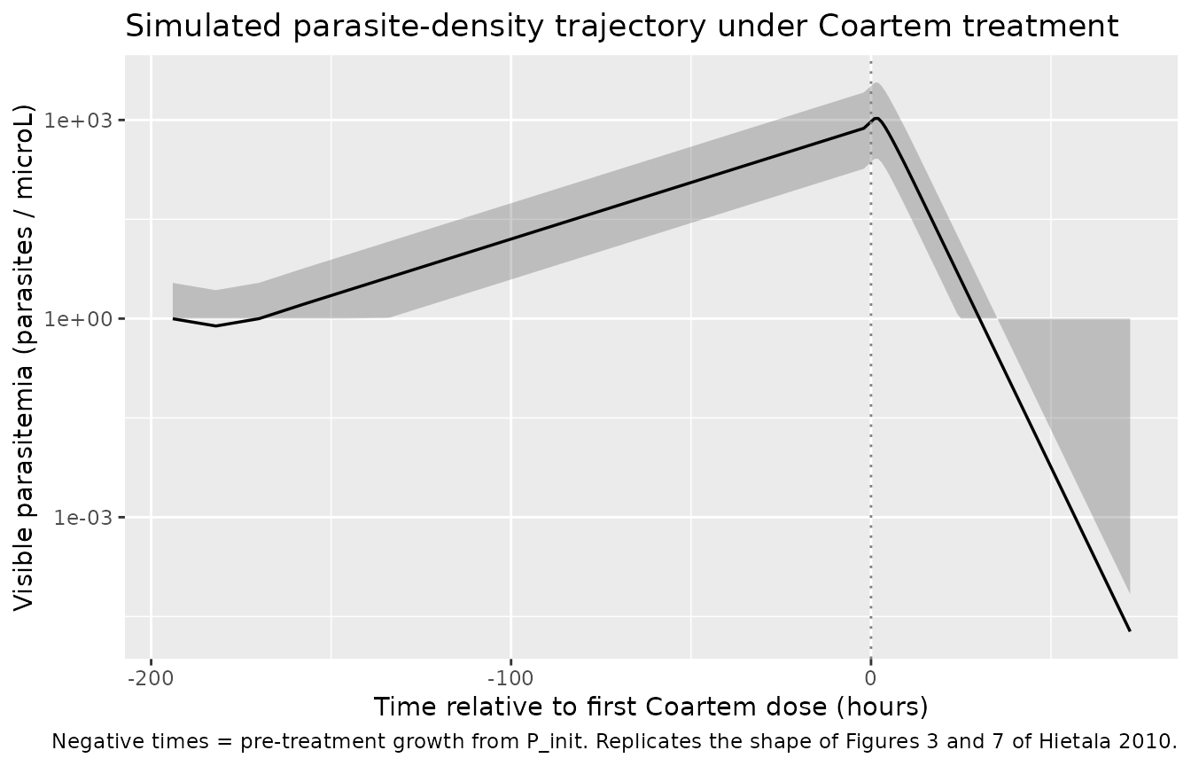
The paper reports a typical predicted parasite clearance time (PCT) of 38 h, against an observed median PCT of 36 h. The PCT is conventionally defined as the time to drop below the limit of microscopic detection (~10 parasites/microL); below summarise the typical-subject crossing time.
mod_pd_typical    <- rxode2::zeroRe(mod_pd)
typical_subjects  <- data.frame(id = 1L, WT = 14, treatment = "Typical (WT = 14 kg)")
events_pd_typical <- build_pd_events(typical_subjects, obs_times_pd, dose_times_pd)
sim_pd_typical    <- rxode2::rxSolve(mod_pd_typical, events = events_pd_typical,
                                     keep = c("WT", "OCC", "treatment")) |>
  as.data.frame()
#> ℹ omega/sigma items treated as zero: 'etalcl', 'etalcl_dihydroart', 'etap_init'

post_dose <- sim_pd_typical |>
  dplyr::filter(!is.na(visibleParasitemia), time >= shift) |>
  dplyr::mutate(time_post_dose = time - shift)

# Peak (admission) parasitemia and the time at which the typical trajectory
# falls below 10 parasites/microL
peak     <- max(post_dose$visibleParasitemia, na.rm = TRUE)
below    <- post_dose[post_dose$visibleParasitemia <= 10 &
                        post_dose$time_post_dose > 0, ]
pct_h    <- if (nrow(below) > 0) min(below$time_post_dose) else NA_real_
sprintf("Typical-subject admission parasitemia: %.0f /microL; simulated PCT (time to <= 10 /microL): %.1f h (paper Discussion: 38 h predicted vs 36 h observed)",
        peak, pct_h)
#> [1] "Typical-subject admission parasitemia: 1061 /microL; simulated PCT (time to <= 10 /microL): 22.0 h (paper Discussion: 38 h predicted vs 36 h observed)"
PKNCA validation
Single-dose AUClast / Cmax / Tmax on the first dosing interval (0-8 h) for ARM, DHA, and LUM. The interval window is short on purpose: terminal-phase characterisation (half-life, AUC-inf) of ARM and LUM is not feasible from a six-dose regimen with sampling out to 72 h post first dose, so the comparison against the Hietala 2010 cohort focuses on AUClast within the first dosing interval.
sim_arm_nca <- sim_arm |>
  dplyr::filter(!is.na(Cc), time <= 8) |>
  dplyr::select(id, time, Cc, treatment)
sim_dha_nca <- sim_arm |>
  dplyr::filter(!is.na(Cc_dihydroart), time <= 8) |>
  dplyr::select(id, time, treatment, Cc = Cc_dihydroart)

dose_arm_nca <- events_arm |>
  dplyr::filter(evid == 1, time == 0) |>
  dplyr::select(id, time, amt, treatment)

intervals_short <- data.frame(start = 0, end = 8, cmax = TRUE, tmax = TRUE,
                              auclast = TRUE)

nca_arm_obj  <- PKNCA::PKNCAconc(sim_arm_nca, Cc ~ time | treatment + id)
nca_dha_obj  <- PKNCA::PKNCAconc(sim_dha_nca, Cc ~ time | treatment + id)
nca_dose_obj <- PKNCA::PKNCAdose(dose_arm_nca, amt ~ time | treatment + id)

nca_arm_res  <- PKNCA::pk.nca(PKNCA::PKNCAdata(nca_arm_obj, nca_dose_obj,
                                               intervals = intervals_short))
nca_dha_res  <- PKNCA::pk.nca(PKNCA::PKNCAdata(nca_dha_obj, nca_dose_obj,
                                               intervals = intervals_short))

knitr::kable(summary(nca_arm_res), caption = "ARM first-interval NCA (interval 0-8 h).")| start | end | treatment | N | auclast | cmax | tmax |
|---|---|---|---|---|---|---|
| 0 | 8 | Coartem (6 doses) | 40 | 1580 [31.8] | 523 [24.5] | 1.00 [1.00, 1.00] |
| start | end | treatment | N | auclast | cmax | tmax |
|---|---|---|---|---|---|---|
| 0 | 8 | Coartem (6 doses) | 40 | 595 [51.1] | 164 [51.5] | 2.00 [1.00, 2.00] |
sim_lum_nca <- sim_lum |>
  dplyr::filter(!is.na(Cc), time <= 72) |>
  dplyr::select(id, time, Cc, treatment)
dose_lum_nca <- events_lum |>
  dplyr::filter(evid == 1, time == 0) |>
  dplyr::select(id, time, amt, treatment)

intervals_lum <- data.frame(start = 0, end = 72, cmax = TRUE, tmax = TRUE,
                            auclast = TRUE)

nca_lum_obj  <- PKNCA::PKNCAconc(sim_lum_nca, Cc ~ time | treatment + id)
nca_lum_dose <- PKNCA::PKNCAdose(dose_lum_nca, amt ~ time | treatment + id)
nca_lum_res  <- PKNCA::pk.nca(PKNCA::PKNCAdata(nca_lum_obj, nca_lum_dose,
                                               intervals = intervals_lum))

knitr::kable(summary(nca_lum_res), caption = "LUM cumulative-regimen NCA (interval 0-72 h, including the six-dose pulse train).")| start | end | treatment | N | auclast | cmax | tmax |
|---|---|---|---|---|---|---|
| 0 | 72 | Coartem (6 doses) | 40 | 486000 [59.6] | 11500 [54.6] | 65.2 [63.0, 72.0] |
Assumptions and deviations
-
Concentration units = nM (
nmol/L). The paper reports all ARM / DHA / LUM concentrations in nM (LC-MS/MS for ARM/DHA, SPE / LC / UV for LUM with LLOQ = 47 nM), andunits$concentration = "nmol/L"matches that.checkModelConventions()flags a softdosing_concentrationwarning because the dose unit (mg) and the concentration numerator (nmol) are not dimensionally identical without an explicit molecular-weight conversion; the conversion is performed inline inmodel()(Cc <- 1e6 * central / vc / mw_arm, etc.) using molecular weights MW_ARM = 298.4, MW_DHA = 284.3, MW_LUM = 528.94 g/mol. The warning is therefore expected and not a structural bug. -
Q ARMTable 1 unit. Table 1 prints the artemether intercompartmental clearance asQ ARM (liters/kg), missing the/h. The description column reads “Intercompartment clearance” (a flux), and the value 1.4 is in line with the other CL / Q / V_ARM scales when interpreted as L/h/kg. The model encodes Q/F_ARM = 1.4 L/h/kg accordingly. -
p_initinterpretation. The published equation 1 carriesP_initas an additive term indP_TR / dt, which would be a continuous source rate with units parasites/microL/h. The Methods text describes it as “the introduction of a certain parasitemia (P_init) into the compartment denoted by tiny rings” with units parasites/microL, and Table 3 labels it “Initial parasitemia”. The two readings disagree; the package model adopts the text/table interpretation (initial condition onparasite_tinyrings) because it is dimensionally consistent and the typical-subject simulation reproduces clinically realistic admission parasitemia after the documented 4-cycle pre-dose growth window. A future reader who prefers the equation-1 form can substitutedP_TR/dt = p_init + ...(and drop the initial-condition line) insidemodel(). -
Log-concentration killing numerical guard. The
published
k_ARM = S * log[ARM]formula is undefined at[ARM] = 0and negative at0 < [ARM] < 1nM. The model file gates the killing rate with(Cc > 1)so the contribution is identically zero below 1 nM and a smoothS * log(Cc)above, matching the standard NONMEMIF (CARM .GT. 1)form. This affects only the pre-dose epoch (where ARM = 0 = DHA = 0) and the early absorption / late terminal tails of each dosing cycle. -
Asymptomatic-children parameterisation not encoded.
Hietala 2010 Table 3 reports a separate asymptomatic-cohort
parameterisation (REPL_a = 1 fixed, A_a = 1.01 estimated, sine
modulation active, fitting the same compartmental structure to 104
capillary parasite counts from 11 asymptomatic children).
Hietala_2010_artemether_parasitemiaencodes only the symptomatic-patient column because that is the primary clinical use; a downstream user who needs the asymptomatic case can overriderepl <- 1; amp <- 1.01in a copy of the model. -
Lumefantrine effect not encoded in the PD model.
Hietala 2010 reports that “the introduction of an effect of LUM did not
significantly improve the model fit, and the parameter estimates for LUM
effect could not be estimated” (Results, Pharmacodynamic model). The
companion
Hietala_2010_lumefantrinehandles LUM in isolation; the PD model is driven by ARM / DHA only. -
Milk-intake covariate not encoded in the LUM PK
model. Hietala 2010 tested 200 mL full-fat cow’s milk as a
categorical covariate on the LUM PK parameters; the effect “did not
explain the variability in LUM pharmacokinetics and did not result in an
improvement of the model” (Results) and is documented in
covariatesDataExcludedrather than encoded inmodel(). -
Pre-treatment growth window for PD simulation. The
package model places the parasite population’s introduction at
simulation start (
parasite_tinyrings(0) <- p_init_i); a forward-simulation use of the PD model therefore needs the dosing schedule shifted by 4 * MTT = 194 h so the parasite population can grow to clinically realistic admission parasitemia before drug dosing begins. The vignette helper functions illustrate this shift; a user who supplies their own dataset must apply the same shift to its dose times. -
OCC = 1 default outside dosing intervals. The
simulation pre-dose epoch (in the parasitemia model) is assigned
OCC = 1.(OCC - 1) = 0then collapses the CL/F_ARM time-dependence to the first-dose value, which is the correct extrapolation for the pre-dose interval (no doses have been given, so the post-dose 6 clearance value would be biologically nonsensical). The same holds at any user-supplied dataset record whereOCCis missing or set to 1. - Small virtual cohort (n = 40). The vignette uses 40 simulated children rather than the 50 reported in the paper, to keep the render time under the 5-minute pkgdown gate. Population-level summaries (median, 5th-95th percentile bands) are stable at this size for the level of detail shown in the figures.
-
Typical-subject PCT differs from the paper’s stochastic
median PCT. The typical-subject simulation (no IIV) gives a
parasite-clearance time of about 22 h, whereas Hietala 2010 reports a
simulated median PCT of 38 h (vs an observed median of 36 h). The
difference is driven by admission parasitemia: with
p_init = 1and REPL_p = 4 the deterministic typical individual reaches an admission parasitemia at the low end of the clinical range (~1000 /microL vs 2,000-200,000 /microL in the cohort), so the typical individual has less parasite mass to clear and clears faster than the paper’s stochastic median. The paper’s PCT was derived from 1000 stochastic simulations withetap_initlog-normal IIV (CV 119.2%), under which the cohort spans the full clinical range; a user reproducing the paper’s PCT figure should match that simulation design (rxSolvewithnSub~ 1000 and a per-subject random P_init from the log-normal IIV in the model).