Cariprazine, desmethyl-cariprazine and didesmethyl-cariprazine (Periclou 2021)
Source:vignettes/articles/Periclou_2021_cariprazine.Rmd
Periclou_2021_cariprazine.RmdModel and source
- Citation: Periclou A, Phillips L, Ghahramani P, Kapas M, Carrothers T, Khariton T. Population Pharmacokinetics of Cariprazine and its Major Metabolites. Eur J Drug Metab Pharmacokinet. 2021;46(1):53-69. doi:10.1007/s13318-020-00650-4
- Description: Population PK model (final model on the updated dataset) for oral cariprazine and its two active metabolites desmethyl-cariprazine (DCAR) and didesmethyl-cariprazine (DDCAR) in adults with schizophrenia or bipolar mania: three-compartment cariprazine with zero-order input into a depot followed by first-order absorption; cariprazine elimination forms DCAR (two-compartment), DCAR elimination forms DDCAR through a single delay transit compartment (two-compartment DDCAR); body weight, race (Black, Asian, Japanese) and sex covariates, and first-dose shifts on cariprazine Vc/Vp1/Q3 and DCAR Vc/Vp
- Article: Eur J Drug Metab Pharmacokinet 2021;46(1):53-69 (open access)
- Supplement: Electronic Supplementary Material 1 of the article (Supplemental Equation Sets 1-3 and Supplemental Tables 1-4)
Periclou 2021 reports two sets of sequentially fitted parent-metabolite models, and both are packaged:
-
Periclou_2021_cariprazine– the final models on the updated dataset (Table 2, Supplemental Equation Sets 1 and 3). This is the paper’s headline model and the one to use for simulation. -
Periclou_2021_cariprazine_initial– the final models on the initial dataset (Supplemental Equation Set 2, Supplemental Table 3), fitted before the rich-sampling Japanese study A002-A11 was available and restricted to samples collected within 25 h of a dose. It is superseded by the updated model and is included for completeness.
The cariprazine, DCAR and DDCAR models were estimated one after another with the preceding analyte’s individual parameters fixed, and all cariprazine eliminated was assumed to become DCAR and all DCAR eliminated to become DDCAR. The DCAR and DDCAR parameters are therefore apparent values, and each file couples the three analytes into a single ODE system.
Population
The updated model was developed on 2199 adults (18-65 years, mean 39.2 years) from three phase 1 studies, eight phase 2/3 studies and the Japanese open-label study A002-A11, of whom 66% were men. Body weight averaged 78.9 kg (SD 18.7, range 33.1-155.1). The cohort was 45.6% White, 34.9% Black, 14.3% Asian (mainly patients at Indian sites), 1.7% Japanese and 3.5% other race (Supplemental Table 2). Patients had schizophrenia or manic/mixed episodes of bipolar I disorder and received oral cariprazine once daily at 0.5-12.5 mg; data after doses of 15 mg/day or more were excluded. The long-term open-label studies RGH-MD-11 and RGH-MD-17 were held out for external validation. Creatinine clearance and CYP2D6 metaboliser status had no effect on exposure.
The same information is available programmatically via
readModelDb("Periclou_2021_cariprazine")()$population.
Model structure
Supplemental Equation Set 1 and Figure 1 of the paper define nine states:
-
depotreceives the dose as a zero-order input overDUR= 2.57 h and empties intocentralby first-order absorption (Ka). - Cariprazine distributes from
centralto two peripheral compartments (peripheral1throughQ3/F,peripheral2throughQ4/F). - Cariprazine elimination (
CL/Vc) is the formation rate of DCAR incentral_dcar, which exchanges withperipheral1_dcar. - DCAR elimination (
DCL/DVc) feeds a single delay compartment,transit1, which empties intocentral_ddcaratDDKtr= 0.0269 1/h. The delay reflects that only 2.6% of patients had measurable DDCAR before day 2. - DDCAR exchanges with
peripheral1_ddcarand is eliminated byDDCL/DDVc.
Because the phase 2/3 studies did not sample after the first dose,
the authors added a first-dose shift FD (1
for concentrations after the first dose, 0 otherwise) on cariprazine
Vc/F, VP1/F and Q3/F and on DCAR
Vc/F and Vp/F. The packaged model builds
FD internally from dosenum(), so no data
column is needed: it equals 1 until the second dose is given.
Dose records must use rate = -2 so that rxode2 applies
dur(depot); a dose without it enters the depot as a
bolus.
mod <- readModelDb("Periclou_2021_cariprazine")
mod_typ <- rxode2::zeroRe(rxode2::rxode2(mod))
#> ℹ parameter labels from comments will be replaced by 'label()'

# Molar-to-mass factors (ng/mL per nM) implied by the paper's own tables:
# Supplemental Table 4 (ng/mL) divided by Table 3 (nM) gives 295 / 690.2,
# 78.0 / 188.7 and 629 / 1573.8, i.e. molecular weights of 427.4, 413.4 and
# 399.7 g/mol for cariprazine, DCAR and DDCAR.
mw <- c(CAR = 0.4274, DCAR = 0.4134, DDCAR = 0.3997)

# Event-table builder. Observation rows sit on the ODE state `central` and
# nominate endpoint 1 through dvid; every observation row returns Cc, Cc_dcar
# and Cc_ddcar together.
make_events <- function(id, dose_times, amts, obs_times, covs) {
  ev <- rbind(
    data.frame(id = id, time = dose_times, amt = amts, rate = -2, evid = 1L,
               cmt = "depot", dvid = NA_integer_),
    data.frame(id = id, time = obs_times, amt = NA_real_, rate = NA_real_,
               evid = 0L, cmt = "central", dvid = 1L)
  )
  ev <- ev[order(ev$time, -ev$evid), ]
  cbind(ev, covs[rep(1, nrow(ev)), , drop = FALSE], row.names = NULL)
}

to_nM <- function(sim) {
  # rxSolve() omits the id column when only one subject is solved.
  if (!"id" %in% names(sim)) sim$id <- 1L
  sim |>
    dplyr::transmute(
      id, time,
      CAR = Cc / mw[["CAR"]],
      DCAR = Cc_dcar / mw[["DCAR"]],
      DDCAR = Cc_ddcar / mw[["DDCAR"]],
      Total = CAR + DCAR + DDCAR
    )
}

trap <- function(t, y) sum(diff(t) * (head(y, -1) + tail(y, -1)) / 2)

male_white <- function(WT) {
  data.frame(WT = WT, SEXF = 0, RACE_BLACK = 0, RACE_ASIAN = 0, RACE_JAPANESE = 0)
}
Source trace
Every ini() value carries an in-file comment naming its
source. They are collected here.
| Parameter | Value | Source location |
|---|---|---|
ld1 (DUR) |
log(2.57 h) | Table 2 |
lka (Ka) |
log(0.352 1/h) | Table 2 |
lcl (CL/F) |
log(21.5 L/h) | Table 2; Suppl Eq 10 |
e_wt_cl, e_black_cl,
e_asian_cl, e_japanese_cl
|
0.0946, -0.0907, -0.178, -0.111 | Table 2; Suppl Eq 10 |
lvc (Vc/F) |
log(266 L) | Table 2; Suppl Eq 11 |
e_wt_vc, e_fd_vc
|
1.66, 2.84 (fixed) | Table 2; Suppl Eq 11 |
lq (Q3/F), e_fd_q
|
log(0.431 L/h) fixed, 39.4 fixed | Table 2; Suppl Eq 12 |
lvp (VP1/F), e_fd_vp
|
log(149 L) fixed, 2.61 fixed | Table 2; Suppl Eq 13 |
lq2 (Q4/F), lvp2 (VP2/F) |
log(100 L/h), log(501 L), both fixed | Table 2 |
lcl_dcar (DCL/F) |
log(77.3 L/h) | Table 2; Suppl Eq 14 |
e_wt_cl_dcar, e_black_cl_dcar,
e_asian_cl_dcar, e_japanese_cl_dcar,
e_sexf_cl_dcar
|
0.578, 0.249, -0.0861, -0.145, -0.160 | Table 2; Suppl Eq 14 |
lvc_dcar (DVc/F), e_wt_vc_dcar,
e_fd_vc_dcar
|
log(128 L), 1.18, 1.27 fixed | Table 2; Suppl Eq 15 |
lq_dcar (DQ/F) |
log(78.5 L/h) | Table 2 |
lvp_dcar (DVp/F), e_fd_vp_dcar
|
log(347 L), 0.535 fixed | Table 2; Suppl Eq 16 |
lcl_ddcar (DDCL/F) |
log(9.24 L/h) | Table 2; Suppl Eq 17 |
e_wt_cl_ddcar, e_black_cl_ddcar,
e_asian_cl_ddcar, e_japanese_cl_ddcar
|
0.427, 0.547, -0.194, -0.156 | Table 2; Suppl Eq 17 |
lvc_ddcar (DDVc/F) |
log(1310 L) | Table 2; Suppl Eq 18 |
e_wt_vc_ddcar, e_black_vc_ddcar,
e_asian_vc_ddcar, e_japanese_vc_ddcar
|
0.881, 0.676, -0.240, 0.0888 | Table 2; Suppl Eq 18 |
lq_ddcar (DDQ/F), lvp_ddcar (DDVp/F) |
log(0.386 L/h), log(258 L), both fixed | Table 2 |
lktr (DDKtr) |
log(0.0269 1/h) fixed | Table 2 |
etalka, etalcl, etalvc
|
0.8723, 0.0998, 0.7830 | Table 2 IIV 118%, 32.4%, 109% CV; log(1 + CV^2)
|
etalcl_dcar, etalvc_dcar
|
0.1653, 0.8426 | Table 2 IIV 42.4%, 115% CV |
etalcl_ddcar, etalvc_ddcar
|
0.2848, 0.4733 | Table 2 IIV 57.4%, 77.8% CV |
propSd, propSd_dcar,
propSd_ddcar
|
0 (fixed) | not reported (Table 2 footnote f) |
ODEs d/dt(depot) …
d/dt(peripheral1_ddcar)
|
n/a | Suppl Equation Set 1, Eqs 1-9; Figure 1 |
dur(depot) zero-order input |
n/a | Suppl Eq 1 (‘initial condition of Dose/DUR’); Figure 1 ‘R0 = Dose/DUR’ |
First-dose indicator fd
|
n/a | Suppl Equation Set 3 definition of FD; Section 3.2.2 |
The initial-dataset model
(Periclou_2021_cariprazine_initial) takes its values from
Supplemental Table 3 and its covariate equations from Supplemental
Equations A1-A6, line by line as documented in that file.
Typical-patient profiles (replicates Figure 5)
The paper’s Section 3.6 describes Figure 5 as a simulation of an
“overall typical patient (79 kg, Caucasian/white adult male)”. Solving
the model at 79 kg puts cariprazine about 8.5% above every Figure 5a
point from 2 to 12 h, whereas at 84 kg – the typical
Caucasian male the paper uses in Figures 6 and 7 – the same points agree
to within 3% for both cariprazine and DCAR. Weight scales cariprazine
Vc/F with exponent 1.66, so that is exactly the size of
offset a 5 kg difference produces. Figure 5 is therefore replicated at
84 kg. The figure values below were read from the published figure by
the maintainers (about +/-0.1 nM in panel a, +/-1 nM in panel b and
+/-10 nM*h in panel c).
fig5a <- tibble::tribble(
  ~analyte, ~time, ~conc,
  "CAR", 1, 0.72, "CAR", 2, 2.55, "CAR", 3, 4.82, "CAR", 4, 6.32,
  "CAR", 6, 7.50, "CAR", 8, 7.56, "CAR", 12, 6.87, "CAR", 24, 2.24,
  "DCAR", 2, 0.10, "DCAR", 3, 0.28, "DCAR", 4, 0.51, "DCAR", 6, 0.88,
  "DCAR", 8, 1.11, "DCAR", 12, 1.31, "DCAR", 24, 1.12,
  "DDCAR", 12, 0.05, "DDCAR", 24, 0.48
)
fig5b <- tibble::tribble(
  ~analyte, ~day, ~conc,
  "CAR", 1.5, 14.1, "CAR", 2, 10.0, "CAR", 3, 5.9, "CAR", 4, 3.3, "CAR", 5, 2.0,
  "CAR", 6, 1.3,
  "DDCAR", 2, 57.1, "DDCAR", 3, 54.9, "DDCAR", 4, 50.8, "DDCAR", 5, 45.7,
  "DDCAR", 6, 40.4, "DDCAR", 8, 31.4, "DDCAR", 10, 23.8, "DDCAR", 12, 17.8,
  "DDCAR", 14, 13.4, "DDCAR", 21, 5.0, "DDCAR", 28, 2.8
)
fig5c <- tibble::tribble(
  ~analyte, ~day, ~auc,
  "CAR", 7, 627, "CAR", 14, 655, "CAR", 84, 655,
  "DCAR", 7, 224, "DCAR", 14, 232, "DCAR", 84, 232,
  "DDCAR", 7, 471, "DDCAR", 14, 1078, "DDCAR", 21, 1290, "DDCAR", 28, 1370,
  "DDCAR", 84, 1430,
  "Total", 7, 1186, "Total", 14, 1825, "Total", 21, 2045, "Total", 28, 2117,
  "Total", 84, 2185
)
Figure 5a: first 6 mg dose
ev_sd <- make_events(1L, 0, 6, c(0, seq(0.25, 24, by = 0.25)), male_white(84))
sd84 <- rxode2::rxSolve(mod_typ, ev_sd, returnType = "data.frame") |> to_nM()
#> ℹ omega/sigma items treated as zero: 'etalka', 'etalcl', 'etalvc', 'etalcl_dcar', 'etalvc_dcar', 'etalcl_ddcar', 'etalvc_ddcar'

sd84 |>
  tidyr::pivot_longer(c(CAR, DCAR, DDCAR, Total), names_to = "analyte", values_to = "conc") |>
  ggplot(aes(time, conc, colour = analyte)) +
  geom_line() +
  geom_point(data = fig5a, shape = 1, size = 2) +
  labs(x = "Time after first dose (h)", y = "Concentration (nM)", colour = NULL,
       title = "Figure 5a: single 6 mg dose, typical 84 kg White male",
       caption = "Lines: packaged model. Open circles: values read from Figure 5a of Periclou 2021.")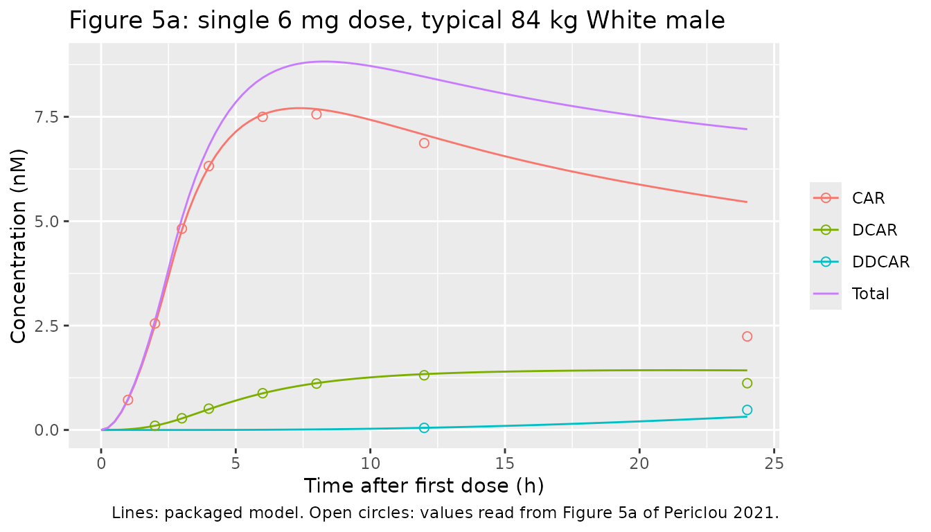
chk5a <- fig5a |>
  dplyr::rowwise() |>
  dplyr::mutate(model = sd84[[analyte]][which.min(abs(sd84$time - time))]) |>
  dplyr::ungroup() |>
  dplyr::mutate(pct_diff = 100 * (model - conc) / conc)
knitr::kable(chk5a, digits = 2, caption = "Model vs Figure 5a (nM).")| analyte | time | conc | model | pct_diff |
|---|---|---|---|---|
| CAR | 1 | 0.72 | 0.73 | 1.19 |
| CAR | 2 | 2.55 | 2.52 | -1.23 |
| CAR | 3 | 4.82 | 4.79 | -0.64 |
| CAR | 4 | 6.32 | 6.31 | -0.23 |
| CAR | 6 | 7.50 | 7.55 | 0.71 |
| CAR | 8 | 7.56 | 7.69 | 1.66 |
| CAR | 12 | 6.87 | 7.07 | 2.93 |
| CAR | 24 | 2.24 | 5.46 | 143.69 |
| DCAR | 2 | 0.10 | 0.10 | 1.90 |
| DCAR | 3 | 0.28 | 0.28 | -1.29 |
| DCAR | 4 | 0.51 | 0.50 | -2.69 |
| DCAR | 6 | 0.88 | 0.88 | -0.24 |
| DCAR | 8 | 1.11 | 1.12 | 0.97 |
| DCAR | 12 | 1.31 | 1.34 | 2.12 |
| DCAR | 24 | 1.12 | 1.43 | 27.41 |
| DDCAR | 12 | 0.05 | 0.05 | 2.65 |
| DDCAR | 24 | 0.48 | 0.32 | -33.72 |
# Deterministic typical-value solve, so tight bounds are appropriate. Measured
# at authoring: cariprazine within 3% at 1-12 h, DCAR within 3% at 4-12 h.
# The 24 h points are a documented deviation (see Assumptions and deviations)
# and are excluded from the gate, as is DCAR at 2-3 h where the figure values
# (0.10 and 0.28 nM) sit at the resolution of the digitisation.
g_car <- chk5a$analyte == "CAR" & chk5a$time <= 12
g_dcar <- chk5a$analyte == "DCAR" & chk5a$time >= 4 & chk5a$time <= 12
stopifnot(
  sum(g_car) == 7, sum(g_dcar) == 4,
  max(abs(chk5a$pct_diff[g_car])) < 8,
  max(abs(chk5a$pct_diff[g_dcar])) < 8
)
Figure 5b: washout after the last dose at steady state
ev_ss <- make_events(1L, seq(0, 83 * 24, by = 24), 6,
                     c(0, seq(83 * 24, 111 * 24, by = 0.5)), male_white(84))
ss84 <- rxode2::rxSolve(mod_typ, ev_ss, returnType = "data.frame") |>
  to_nM() |>
  dplyr::filter(time >= 83 * 24) |>
  dplyr::mutate(day = (time - 83 * 24) / 24)
#> ℹ omega/sigma items treated as zero: 'etalka', 'etalcl', 'etalvc', 'etalcl_dcar', 'etalvc_dcar', 'etalcl_ddcar', 'etalvc_ddcar'

ss84 |>
  tidyr::pivot_longer(c(CAR, DCAR, DDCAR, Total), names_to = "analyte", values_to = "conc") |>
  ggplot(aes(day, conc, colour = analyte)) +
  geom_line() +
  geom_point(data = fig5b, shape = 1, size = 2) +
  labs(x = "Time after the last of 84 daily 6 mg doses (days)", y = "Concentration (nM)",
       colour = NULL, title = "Figure 5b: washout from steady state, typical 84 kg White male",
       caption = "Lines: packaged model. Open circles: values read from Figure 5b of Periclou 2021.")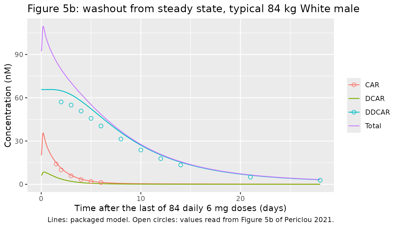
chk5b <- fig5b |>
  dplyr::rowwise() |>
  dplyr::mutate(model = ss84[[analyte]][which.min(abs(ss84$day - day))]) |>
  dplyr::ungroup() |>
  dplyr::mutate(pct_diff = 100 * (model - conc) / conc)
knitr::kable(chk5b, digits = 2, caption = "Model vs Figure 5b (nM).")| analyte | day | conc | model | pct_diff |
|---|---|---|---|---|
| CAR | 1.5 | 14.1 | 14.95 | 6.01 |
| CAR | 2.0 | 10.0 | 11.16 | 11.56 |
| CAR | 3.0 | 5.9 | 6.29 | 6.62 |
| CAR | 4.0 | 3.3 | 3.63 | 10.13 |
| CAR | 5.0 | 2.0 | 2.18 | 8.88 |
| CAR | 6.0 | 1.3 | 1.37 | 5.64 |
| DDCAR | 2.0 | 57.1 | 64.86 | 13.58 |
| DDCAR | 3.0 | 54.9 | 62.09 | 13.10 |
| DDCAR | 4.0 | 50.8 | 57.70 | 13.57 |
| DDCAR | 5.0 | 45.7 | 52.35 | 14.55 |
| DDCAR | 6.0 | 40.4 | 46.68 | 15.56 |
| DDCAR | 8.0 | 31.4 | 35.95 | 14.49 |
| DDCAR | 10.0 | 23.8 | 27.11 | 13.92 |
| DDCAR | 12.0 | 17.8 | 20.36 | 14.36 |
| DDCAR | 14.0 | 13.4 | 15.35 | 14.55 |
| DDCAR | 21.0 | 5.0 | 6.29 | 25.80 |
| DDCAR | 28.0 | 2.8 | 3.15 | 12.67 |
# Cariprazine washout reproduces within about 12% (measured +6% to +12% at
# authoring). DDCAR runs a near-constant 13-16% high over the whole washout
# (26% at day 21, where the figure value is small), the same offset seen in
# its steady-state level (see Figure 5c below), so its shape is reproduced
# and only its level differs.
stopifnot(
  max(abs(chk5b$pct_diff[chk5b$analyte == "CAR"])) < 15,
  abs(median(chk5b$pct_diff[chk5b$analyte == "DDCAR"])) < 25
)
Figure 5c: daily AUC during titration to 6 mg
Figure 5c titrates 1.5, 3 and 4.5 mg on days 1-3 and 6 mg daily thereafter.
amts_tit <- c(1.5, 3, 4.5, rep(6, 81))
ev_tit <- make_events(1L, seq(0, 83 * 24, by = 24), amts_tit,
                      seq(0, 84 * 24, by = 0.25), male_white(84))
tit84 <- rxode2::rxSolve(mod_typ, ev_tit, returnType = "data.frame") |> to_nM()
#> ℹ omega/sigma items treated as zero: 'etalka', 'etalcl', 'etalvc', 'etalcl_dcar', 'etalvc_dcar', 'etalcl_ddcar', 'etalvc_ddcar'

daily_auc <- tit84 |>
  dplyr::mutate(day = pmin(floor(time / 24) + 1, 84)) |>
  dplyr::group_by(day) |>
  dplyr::group_modify(function(d, key) {
    w <- tit84[tit84$time >= (key$day - 1) * 24 & tit84$time <= key$day * 24, ]
    data.frame(CAR = trap(w$time, w$CAR), DCAR = trap(w$time, w$DCAR),
               DDCAR = trap(w$time, w$DDCAR), Total = trap(w$time, w$Total))
  }) |>
  dplyr::ungroup() |>
  tidyr::pivot_longer(-day, names_to = "analyte", values_to = "auc")

ggplot(daily_auc, aes(day, auc, colour = analyte)) +
  geom_line() +
  geom_point(data = fig5c, shape = 1, size = 2) +
  labs(x = "Day of dosing", y = "AUC0-24 (nM*h)", colour = NULL,
       title = "Figure 5c: daily AUC0-24 during titration to 6 mg/day",
       caption = "Lines: packaged model. Open circles: values read from Figure 5c of Periclou 2021.")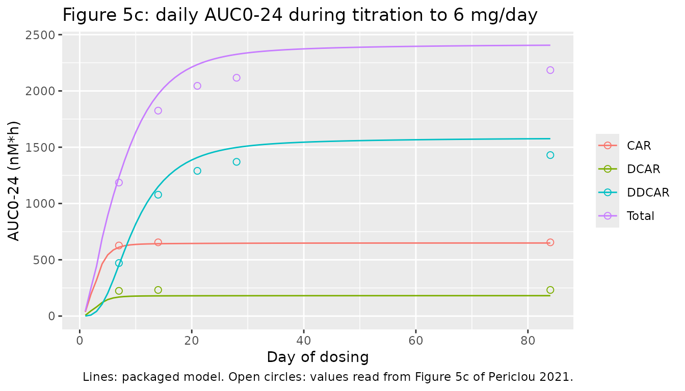
chk5c <- fig5c |>
  dplyr::left_join(daily_auc, by = c("analyte", "day"), suffix = c("_fig", "_model")) |>
  dplyr::mutate(pct_diff = 100 * (auc_model - auc_fig) / auc_fig)
knitr::kable(chk5c, digits = 1, caption = "Model vs Figure 5c (nM*h).")| analyte | day | auc_fig | auc_model | pct_diff |
|---|---|---|---|---|
| CAR | 7 | 627 | 611.5 | -2.5 |
| CAR | 14 | 655 | 642.6 | -1.9 |
| CAR | 84 | 655 | 649.1 | -0.9 |
| DCAR | 7 | 224 | 169.1 | -24.5 |
| DCAR | 14 | 232 | 179.3 | -22.7 |
| DCAR | 84 | 232 | 181.2 | -21.9 |
| DDCAR | 7 | 471 | 453.0 | -3.8 |
| DDCAR | 14 | 1078 | 1149.2 | 6.6 |
| DDCAR | 21 | 1290 | 1408.9 | 9.2 |
| DDCAR | 28 | 1370 | 1497.7 | 9.3 |
| DDCAR | 84 | 1430 | 1575.7 | 10.2 |
| Total | 7 | 1186 | 1233.5 | 4.0 |
| Total | 14 | 1825 | 1971.1 | 8.0 |
| Total | 21 | 2045 | 2234.3 | 9.3 |
| Total | 28 | 2117 | 2325.0 | 9.8 |
| Total | 84 | 2185 | 2406.0 | 10.1 |
# Figure 5c is not internally consistent: its Total curve sits about 130 nM*h
# BELOW the sum of its own CAR + DCAR + DDCAR curves at every day, so only the
# cariprazine curve is gated. At authoring the cariprazine plateau matched
# within 1%.
fig_sum_gap <- with(fig5c, auc[analyte == "Total" & day == 84] -
  sum(auc[analyte %in% c("CAR", "DCAR", "DDCAR") & day == 84]))
stopifnot(
  fig_sum_gap < -100,
  max(abs(chk5c$pct_diff[chk5c$analyte == "CAR"])) < 5
)
Deterministic mass-balance check
The chain assumes that every molecule of cariprazine eliminated
becomes DCAR and every molecule of DCAR eliminated becomes DDCAR, and
the paper’s equations carry amounts in dose units with no
molecular-weight term. At steady state each analyte’s dosing-interval
AUC must therefore equal Dose / CL of that analyte (in
ng*h/mL). This holds for any correct encoding and breaks at once if a
formation or elimination term is mis-wired.
ev_mb <- make_events(1L, seq(0, 139 * 24, by = 24), 6,
                     seq(139 * 24, 140 * 24, by = 0.05), male_white(79))
mb <- rxode2::rxSolve(mod_typ, ev_mb, returnType = "data.frame")
#> ℹ omega/sigma items treated as zero: 'etalka', 'etalcl', 'etalvc', 'etalcl_dcar', 'etalvc_dcar', 'etalcl_ddcar', 'etalvc_ddcar'
mb_tab <- data.frame(
  analyte = c("CAR", "DCAR", "DDCAR"),
  auc_tau = c(trap(mb$time, mb$Cc), trap(mb$time, mb$Cc_dcar), trap(mb$time, mb$Cc_ddcar)),
  dose_over_cl = 6000 / c(21.5, 77.3, 9.24)
) |>
  dplyr::mutate(pct_diff = 100 * (auc_tau - dose_over_cl) / dose_over_cl)
knitr::kable(mb_tab, digits = 2,
caption = "Steady-state AUC over 24 h vs Dose/CL (ng*h/mL), typical 79 kg White male, day 140.")| analyte | auc_tau | dose_over_cl | pct_diff |
|---|---|---|---|
| CAR | 279.07 | 279.07 | 0.00 |
| DCAR | 77.62 | 77.62 | 0.00 |
| DDCAR | 648.96 | 649.35 | -0.06 |
Japanese patients (Supplemental Table 4)
Supplemental Table 4 gives the population-model mean steady-state exposure for the 37 Japanese patients of study A002-A11 at 6 mg/day. Their mean weight is not reported; the paper’s typical Japanese male in Figure 7 weighs 78 kg.
jp <- data.frame(WT = 78, SEXF = 0, RACE_BLACK = 0, RACE_ASIAN = 0, RACE_JAPANESE = 1)
jp_sim <- rxode2::rxSolve(mod_typ, make_events(1L, seq(0, 139 * 24, by = 24), 6,
                                               seq(139 * 24, 140 * 24, by = 0.1), jp),
                          returnType = "data.frame")
#> ℹ omega/sigma items treated as zero: 'etalka', 'etalcl', 'etalvc', 'etalcl_dcar', 'etalvc_dcar', 'etalcl_ddcar', 'etalvc_ddcar'
jp_tab <- data.frame(
  analyte = c("CAR", "DCAR", "DDCAR"),
  model_auc = c(trap(jp_sim$time, jp_sim$Cc), trap(jp_sim$time, jp_sim$Cc_dcar),
                trap(jp_sim$time, jp_sim$Cc_ddcar)),
  suppl_table4_mean_auc = c(306, 105, 784)
) |>
  dplyr::mutate(pct_diff = 100 * (model_auc - suppl_table4_mean_auc) / suppl_table4_mean_auc)
knitr::kable(jp_tab, digits = 1,
caption = "Typical Japanese male (78 kg) vs Supplemental Table 4 popPK mean AUC0-24 (ng*h/mL).")| analyte | model_auc | suppl_table4_mean_auc | pct_diff |
|---|---|---|---|
| CAR | 314.3 | 306 | 2.7 |
| DCAR | 91.5 | 105 | -12.9 |
| DDCAR | 772.9 | 784 | -1.4 |
# Cariprazine and DDCAR carry no sex effect, so the typical male should sit
# near the Japanese mean (measured +2.7% and -1.4%). DCAR clearance is 16%
# lower in women, and the Japanese cohort was not all male, so the DCAR row
# is shown but not gated.
stopifnot(max(abs(jp_tab$pct_diff[jp_tab$analyte != "DCAR"])) < 10)
Covariate effects on total exposure (Figure 4)
The paper reports that every covariate-related change in steady-state Total CAR exposure was within 36% of its comparator (White or Other for race, male for sex). The typical-value ratios below are for a 79 kg patient.
ss_total_auc <- function(covs) {
  s <- rxode2::rxSolve(mod_typ, make_events(1L, seq(0, 139 * 24, by = 24), 6,
                                            seq(139 * 24, 140 * 24, by = 0.1), covs),
                       returnType = "data.frame") |> to_nM()
  trap(s$time, s$Total)
}
ref <- ss_total_auc(male_white(79))
#> ℹ omega/sigma items treated as zero: 'etalka', 'etalcl', 'etalvc', 'etalcl_dcar', 'etalvc_dcar', 'etalcl_ddcar', 'etalvc_ddcar'
groups <- list(
  Black = data.frame(WT = 79, SEXF = 0, RACE_BLACK = 1, RACE_ASIAN = 0, RACE_JAPANESE = 0),
  Asian = data.frame(WT = 79, SEXF = 0, RACE_BLACK = 0, RACE_ASIAN = 1, RACE_JAPANESE = 0),
  Japanese = data.frame(WT = 79, SEXF = 0, RACE_BLACK = 0, RACE_ASIAN = 0, RACE_JAPANESE = 1),
  Female = data.frame(WT = 79, SEXF = 1, RACE_BLACK = 0, RACE_ASIAN = 0, RACE_JAPANESE = 0)
)
fig4 <- data.frame(group = names(groups),
                   ratio_total_auc = vapply(groups, ss_total_auc, numeric(1)) / ref)
#> ℹ omega/sigma items treated as zero: 'etalka', 'etalcl', 'etalvc', 'etalcl_dcar', 'etalvc_dcar', 'etalcl_ddcar', 'etalvc_ddcar'
#> ℹ omega/sigma items treated as zero: 'etalka', 'etalcl', 'etalvc', 'etalcl_dcar', 'etalvc_dcar', 'etalcl_ddcar', 'etalvc_ddcar'
#> ℹ omega/sigma items treated as zero: 'etalka', 'etalcl', 'etalvc', 'etalcl_dcar', 'etalvc_dcar', 'etalcl_ddcar', 'etalvc_ddcar'
#> ℹ omega/sigma items treated as zero: 'etalka', 'etalcl', 'etalvc', 'etalcl_dcar', 'etalvc_dcar', 'etalcl_ddcar', 'etalvc_ddcar'
knitr::kable(fig4, digits = 3, caption = "Typical-value ratio of steady-state Total CAR AUC0-24 to a 79 kg White male.")| group | ratio_total_auc | |
|---|---|---|
| Black | Black | 0.778 |
| Asian | Asian | 1.223 |
| Japanese | Japanese | 1.168 |
| Female | Female | 1.015 |
The directions match Figure 4 of the paper: lower exposure in Black patients, higher in Asian and Japanese patients, and higher in women.
Population simulation and NCA (Table 3)
Table 3 summarises individual steady-state exposure at 6 mg/day, computed from each patient’s post hoc parameters. A virtual cohort of 200 patients is drawn from the Supplemental Table 2 demographics and dosed for 12 weeks.
set.seed(20211103)
n_sub <- 200
draw_wt <- function(n) {
  # Reject-and-redraw inside the observed range rather than clamping.
  w <- rnorm(n, 78.9, 18.7)
  bad <- w < 33.1 | w > 155.1
  while (any(bad)) {
    w[bad] <- rnorm(sum(bad), 78.9, 18.7)
    bad <- w < 33.1 | w > 155.1
  }
  w
}
race <- sample(c("White", "Black", "Asian", "Japanese", "Other"), n_sub, replace = TRUE,
               prob = c(45.6, 34.9, 14.3, 1.7, 3.5))
cohort <- data.frame(
  id = seq_len(n_sub), WT = draw_wt(n_sub), SEXF = rbinom(n_sub, 1, 0.336),
  RACE_BLACK = as.integer(race == "Black"), RACE_ASIAN = as.integer(race == "Asian"),
  RACE_JAPANESE = as.integer(race == "Japanese")
)
events <- do.call(rbind, lapply(seq_len(n_sub), function(i) {
  make_events(i, seq(0, 83 * 24, by = 24), 6,
              c(0, seq(83 * 24, 84 * 24, by = 0.5)), cohort[i, -1])
})) |>
  dplyr::mutate(treatment = "6 mg QD")
stopifnot(!anyDuplicated(events[, c("id", "time", "evid")]))
sim <- rxode2::rxSolve(mod, events = events, keep = "treatment", returnType = "data.frame")
#> ℹ parameter labels from comments will be replaced by 'label()'
sim_nM <- sim |>
  dplyr::transmute(
    id, time, treatment,
    CAR = Cc / mw[["CAR"]], DCAR = Cc_dcar / mw[["DCAR"]], DDCAR = Cc_ddcar / mw[["DDCAR"]]
  ) |>
  tidyr::pivot_longer(c(CAR, DCAR, DDCAR), names_to = "analyte", values_to = "Cc")

sim_nM |>
  dplyr::filter(time >= 83 * 24) |>
  dplyr::group_by(analyte, time) |>
  dplyr::summarise(Q05 = quantile(Cc, 0.05), Q50 = median(Cc), Q95 = quantile(Cc, 0.95),
                   .groups = "drop") |>
  ggplot(aes(time - 83 * 24, Q50)) +
  geom_ribbon(aes(ymin = Q05, ymax = Q95), alpha = 0.25) +
  geom_line() +
  facet_wrap(~analyte, scales = "free_y") +
  labs(x = "Time after the 84th daily 6 mg dose (h)", y = "Concentration (nM)",
       title = "Simulated steady-state profiles (median, 5th-95th percentile)")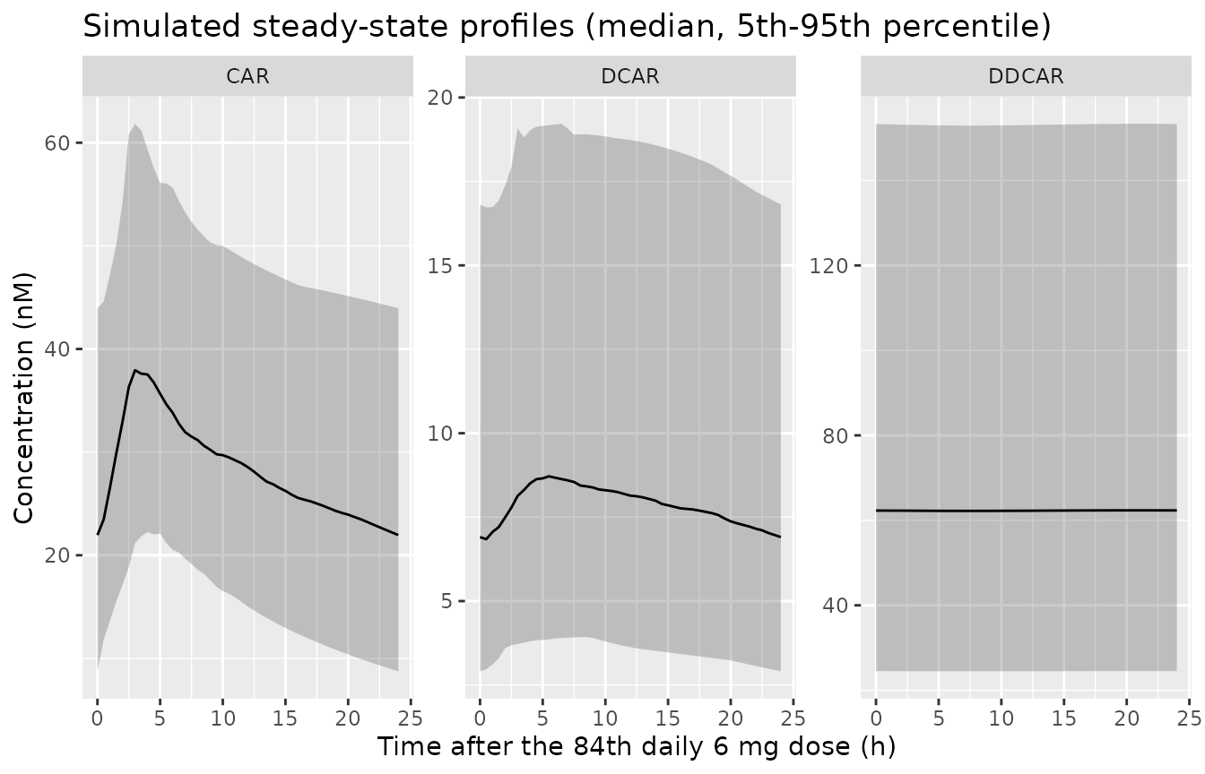
sim_nca <- sim_nM |>
  dplyr::filter(!is.na(Cc)) |>
  dplyr::select(id, time, Cc, treatment, analyte)
conc_obj <- PKNCA::PKNCAconc(sim_nca, Cc ~ time | treatment + analyte + id)
dose_df <- events |>
  dplyr::filter(evid == 1) |>
  dplyr::select(id, time, amt, treatment)
dose_obj <- PKNCA::PKNCAdose(dose_df, amt ~ time | treatment + id)
intervals <- data.frame(start = 83 * 24, end = 84 * 24,
                        cmax = TRUE, cmin = TRUE, auclast = TRUE)
nca_res <- PKNCA::pk.nca(PKNCA::PKNCAdata(conc_obj, dose_obj, intervals = intervals))
Comparison against published steady-state exposure
ncaComparisonTable() compares the simulated median with
the Table 3 median.
published <- tibble::tribble(
  ~treatment, ~analyte, ~cmax, ~cmin, ~auclast,
  "6 mg QD", "CAR", 35.4, 19.9, 641.0,
  "6 mg QD", "DCAR", 8.1, 6.1, 171.1,
  "6 mg QD", "DDCAR", 55.3, 55.3, 1325.9
)
cmp <- nlmixr2lib::ncaComparisonTable(
  simulated = nca_res,
  reference = published,
  by = c("treatment", "analyte"),
  units = c(cmax = "nM", cmin = "nM", auclast = "nM*h"),
  tolerance_pct = 20
)
knitr::kable(cmp, caption = "Simulated vs Table 3 median steady-state exposure at 6 mg/day. * differs from reference by >20%.")| NCA parameter | treatment | analyte | Reference | Simulated | % diff |
|---|---|---|---|---|---|
| Cmax (nM) | 6 mg QD | CAR | 35.4 | 39.5 | +11.4% |
| Cmax (nM) | 6 mg QD | DCAR | 8.1 | 8.83 | +9.0% |
| Cmax (nM) | 6 mg QD | DDCAR | 55.3 | 62.4 | +12.8% |
| Cmin (nM) | 6 mg QD | CAR | 19.9 | 22 | +10.3% |
| Cmin (nM) | 6 mg QD | DCAR | 6.1 | 6.84 | +12.2% |
| Cmin (nM) | 6 mg QD | DDCAR | 55.3 | 62.2 | +12.5% |
| AUClast (nM*h) | 6 mg QD | CAR | 641 | 682 | +6.4% |
| AUClast (nM*h) | 6 mg QD | DCAR | 171 | 188 | +9.9% |
| AUClast (nM*h) | 6 mg QD | DDCAR | 1330 | 1490 | +12.8% |
sim_med <- as.data.frame(nca_res$result) |>
  dplyr::filter(PPTESTCD %in% c("cmax", "auclast")) |>
  dplyr::group_by(analyte, PPTESTCD) |>
  dplyr::summarise(sim = median(PPORRES), .groups = "drop") |>
  dplyr::left_join(
    published |> tidyr::pivot_longer(c(cmax, auclast), names_to = "PPTESTCD", values_to = "ref") |>
      dplyr::select(analyte, PPTESTCD, ref),
    by = c("analyte", "PPTESTCD")
  ) |>
  dplyr::mutate(pct_diff = 100 * (sim - ref) / ref)
# Centre-of-distribution gate on a random cohort. With a 1500-subject cohort
# the model medians sat 8-15% above Table 3 for all three analytes (Table 3
# is built from post hoc estimates of 2599 patients, not from fresh draws);
# 30% absorbs the cohort-to-cohort spread of a 200-subject median while still
# failing on a mis-transcribed clearance or a dose/unit error.
stopifnot(nrow(sim_med) == 6, all(abs(sim_med$pct_diff) < 30))
Table 3 lists identical Cmax,ss and Cmin,ss statistics for DDCAR (mean 65.6, median 55.3 nM in both rows), which is not possible for a drug with any within-interval fluctuation; the DDCAR Cmin,ss reference above is therefore the paper’s Cmax,ss value repeated, and that row should be read with this in mind. DDCAR does fluctuate little over a dosing interval, so the two numbers are close in the simulation too.
Initial-dataset model
The initial-dataset model has a two-compartment cariprazine and one-compartment DCAR and DDCAR, with ideal body weight (reference 64.5 kg), age, race and sex covariates entering mostly as additive shifts. It was fitted only to samples within 25 h of a dose, so its terminal phases are not supported beyond that window. The panel below compares the two models for a typical 40-year-old White man (79 kg, ideal body weight 64.5 kg) after the first dose and on day 84.
mod_init_typ <- rxode2::zeroRe(rxode2::rxode2(readModelDb("Periclou_2021_cariprazine_initial")))
#> ℹ parameter labels from comments will be replaced by 'label()'
cov_both <- data.frame(WT = 79, IBW = 64.5, AGE = 40, SEXF = 0, RACE_BLACK = 0,
                       RACE_ASIAN = 0, RACE_JAPANESE = 0)
obs_cmp <- c(seq(0, 24, by = 0.25), seq(83 * 24, 84 * 24, by = 0.25))
ev_cmp <- make_events(1L, seq(0, 83 * 24, by = 24), 6, obs_cmp, cov_both)
cmp_models <- dplyr::bind_rows(
  rxode2::rxSolve(mod_typ, ev_cmp, returnType = "data.frame") |> to_nM() |>
    dplyr::mutate(model = "Updated (final)"),
  rxode2::rxSolve(mod_init_typ, ev_cmp, returnType = "data.frame") |> to_nM() |>
    dplyr::mutate(model = "Initial dataset")
) |>
  dplyr::mutate(period = ifelse(time < 24.5, "Day 1", "Day 84"),
                tad = ifelse(time < 24.5, time, time - 83 * 24)) |>
  tidyr::pivot_longer(c(CAR, DCAR, DDCAR), names_to = "analyte", values_to = "conc")
#> ℹ omega/sigma items treated as zero: 'etalka', 'etalcl', 'etalvc', 'etalcl_dcar', 'etalvc_dcar', 'etalcl_ddcar', 'etalvc_ddcar'
#> ℹ omega/sigma items treated as zero: 'etalka', 'etalcl', 'etalvc', 'etalcl_dcar', 'etalvc_dcar', 'etalcl_ddcar', 'etalvc_ddcar'
ggplot(cmp_models, aes(tad, conc, colour = model)) +
  geom_line() +
  facet_grid(analyte ~ period, scales = "free_y") +
  labs(x = "Time after dose (h)", y = "Concentration (nM)", colour = NULL,
       title = "Initial-dataset vs updated model, 6 mg once daily")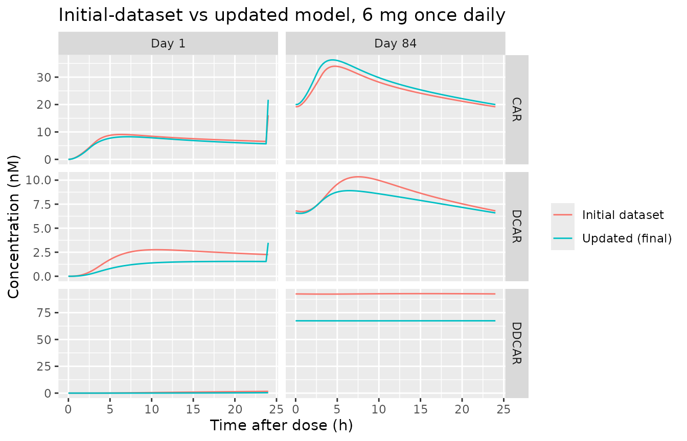
ev_mbi <- make_events(1L, seq(0, 139 * 24, by = 24), 6,
                      seq(139 * 24, 140 * 24, by = 0.05), cov_both)
mbi <- rxode2::rxSolve(mod_init_typ, ev_mbi, returnType = "data.frame")
#> ℹ omega/sigma items treated as zero: 'etalka', 'etalcl', 'etalvc', 'etalcl_dcar', 'etalvc_dcar', 'etalcl_ddcar', 'etalvc_ddcar'
mbi_tab <- data.frame(
  analyte = c("CAR", "DCAR", "DDCAR"),
  auc_tau = c(trap(mbi$time, mbi$Cc), trap(mbi$time, mbi$Cc_dcar), trap(mbi$time, mbi$Cc_ddcar)),
  dose_over_cl = 6000 / c(22.8, 70.9, 6.74)
) |>
  dplyr::mutate(pct_diff = 100 * (auc_tau - dose_over_cl) / dose_over_cl)
knitr::kable(mbi_tab, digits = 2,
caption = "Initial-dataset model: steady-state AUC over 24 h vs Dose/CL (ng*h/mL) at the reference covariates.")| analyte | auc_tau | dose_over_cl | pct_diff |
|---|---|---|---|
| CAR | 263.16 | 263.16 | 0 |
| DCAR | 84.63 | 84.63 | 0 |
| DDCAR | 890.17 | 890.21 | 0 |
Assumptions and deviations
- Residual error is not reported. Table 2 footnote f says residual variability was estimated separately for the phase 1 and phase 2/3 studies, but neither the error model nor its values appear in the paper or supplement. Both packaged models carry proportional errors fixed to zero, so they simulate typical and between-subject variability only and are not suitable for re-estimation as distributed.
-
IIV variances. Table 2 and Supplemental Table 3
report IIV as %CV; they were converted with
omega^2 = log(1 + CV^2), and no correlations are reported, so the random effects are independent. IIV onKa, cariprazineVc/Fand DCARVc/Fwas estimated from phase 1 patients only (Table 2 footnote b; shrinkage 76.5% onKa); the packaged model applies it to every simulated subject. - Mass chain, no molecular-weight term. The printed equations transfer cariprazine elimination to DCAR, and DCAR elimination to DDCAR, amount for amount, and all DCAR and DDCAR parameters are apparent (Section 2.4.1). The packaged model follows the equations literally, in mg of dose with concentrations in ng/mL. Had the authors instead worked in molar amounts, predicted DCAR and DDCAR concentrations would be 3.3% and 6.6% lower. The paper’s own summary numbers do not settle this: the Figure 5c DDCAR plateau is closer to the molar reading, while the DDCAR-to-cariprazine ratios of the Table 3 means and medians are closer to the mass reading. Either reading is well inside the between-subject variability.
-
First-dose shift.
FDis built inside the model fromdosenum()rather than read from a data column. In a NONMEM dataset the flag switches on the record after which it is set; here it switches at the second dose itself. - Figure 5 typical weight. The text describes the Figure 5 patient as 79 kg, but the first-dose profile reproduces to within 3% only at 84 kg, the typical male of Figures 6 and 7, so Figure 5 is replicated at 84 kg.
- Figure 5a at 24 h is not reproduced. At 24 h after the first dose the model gives 5.5 nM cariprazine, 1.4 nM DCAR and 0.3 nM DDCAR, against 2.2, 1.1 and 0.5 nM in the figure, while every earlier point agrees closely. With Q4/F = 100 L/h and VP2/F = 501 L the second peripheral compartment re-equilibrates within hours and the first-dose Vc/F is 1021 L, so no reading of the printed parameters produces the figure’s 3-fold fall between 12 and 24 h. Placing the first-dose shift on VP2/F instead of VP1/F, or switching it off over the 12-24 h interval as a NONMEM record at 24 h would, does not reproduce it either. The deviation is recorded and excluded from the gate.
- Figure 5 metabolite curves. Figure 5c’s Total curve sits about 130 nMh below the sum of its own three analyte curves, and its DCAR plateau (232 nMh) cannot be reconciled with the DCAR concentrations of Figure 5b (about 5.5-7.8 nM, i.e. 130-190 nMh per day). At steady state the model gives DCAR 181 nMh and DDCAR 1576 nM*h for the 84 kg patient, against 232 and 1430 in the figure. Only the cariprazine curve, which is consistent across all three panels, is gated on Figure 5.
- Table 3 DDCAR Cmin,ss repeats the Cmax,ss statistics exactly and is taken as printed.
-
Race indicators. In the updated analysis race had
five mutually exclusive levels.
RACE_ASIANis the non-Japanese Asian group (mainly patients at Indian sites) and must be 0 for Japanese patients, who carryRACE_JAPANESE = 1. White and Other form the reference. -
Initial-dataset Equation A6. Supplemental Equation
A6 prints the DDCAR central volume as
2220 + 27.4 x (Age - 40) + 39.7 x (IBW - 64.5) x (1180 x Black), which would remove the ideal-body-weight term entirely for non-Black patients. Supplemental Table 3 lists 1180 L as an “Additional shift in black patients (L)”, so the Black term is encoded as an additive+ 1180 x Black. - Initial-dataset IIV and IBW. The between-subject variances of the initial-dataset model are applied multiplicatively (log-normal) to the additive covariate expressions. The ideal-body-weight formula is not given in the paper.
- Virtual cohort. Body weight was drawn from a normal distribution with the Supplemental Table 2 mean and SD and redrawn inside the observed range; race and sex follow the Supplemental Table 2 proportions. No correlation between weight, sex and race was imposed.
- Errata. No correction or erratum is linked to this article (PMID 33141308) in Europe PMC as of 2026-09-27.