Lenvatinib exposure, serum biomarkers and tumor dynamics (Majid 2024)

Model and source

Majid 2024 reports an integrated exposure-biomarker-tumor modeling framework for lenvatinib in radioiodine-refractory differentiated thyroid cancer (RR-DTC). The authors fitted three models sequentially: a population PK model on 19 pooled studies, then a simultaneous four-biomarker PK/PD model whose drug driver is the post hoc individual daily AUC from the PK fit, then an integrated tumor-growth- inhibition model whose drivers are that same AUC plus the model-predicted Tie-2 and Ang-2 trajectories. Because the fits are sequential and non-hierarchical, the package ships them as separate model files (see vignette("create-model-library") on replicating the author’s structure).

A fourth file ships an alternative reading of the tumor model; the reason is set out in “The tumor-model fork” below and in the Errata.

model_files <- c(
  "Majid_2024_lenvatinib",
  "Majid_2024_lenvatinib_biomarkers",
  "Majid_2024_lenvatinib_tumor",
  "Majid_2024_lenvatinib_tumor_asdeposited"
)
mod_pk    <- readModelDb("Majid_2024_lenvatinib")
mod_bm    <- readModelDb("Majid_2024_lenvatinib_biomarkers")
mod_tumA  <- readModelDb("Majid_2024_lenvatinib_tumor")
mod_tumB  <- readModelDb("Majid_2024_lenvatinib_tumor_asdeposited")

Citation: Majid O, Hayato S, Sreerama Reddy SH, Lalovic B, Hihara T, Hoshi T, Funahashi Y, Aluri J, Takenaka O, Yasuda S, Hussein Z. Population pharmacokinetic-pharmacodynamic modeling of serum biomarkers as predictors of tumor dynamics following lenvatinib treatment in patients with radioiodine-refractory differentiated thyroid cancer (RR-DTC). CPT Pharmacometrics Syst Pharmacol. 2024;13(6):954-969. doi:10.1002/psp4.13130. Structural model updated from Gupta A, et al. Br J Clin Pharmacol. 2016;81(6):1124-1133; see modellib(‘Gupta_2016_lenvatinib’).
Article: https://doi.org/10.1002/psp4.13130
Supplement (Tables S1-S4, Figures S1-S9, and Supplementary Texts S1-S6 holding the final NONMEM control streams): available from the article’s Supporting Information section.

Model file	Layer	Source
`Majid_2024_lenvatinib`	3-compartment population PK, N = 1921	Table 1, Text S1
`Majid_2024_lenvatinib_biomarkers`	Simultaneous VEGF / Tie-2 / Ang-2 / FGF-23 indirect response, N = 560	Equations 1-3, Table 2, Text S2
`Majid_2024_lenvatinib_tumor`	Tumor growth inhibition + Tie-2 / Ang-2, N = 558, printed Equations 2 and 4	Equation 4, Table 3
`Majid_2024_lenvatinib_tumor_asdeposited`	Same, transcribed literally from Text S3	Text S3, Table 3

Population

The PK model pools 17,550 lenvatinib plasma concentrations from 1921 subjects across 19 phase 1-3 studies: 534 with HCC, 542 with DTC, 491 with RCC, 155 with other solid tumors, and 199 healthy volunteers. Median body weight 73.2 kg (range 32.6-190), median age 61.0 years (range 18-92), 32.2% female, 61.6% White. Doses ranged 3.2-32 mg orally, as capsule (1561 subjects) or tablet (Table S2).

The two PK/PD sub-populations are smaller and are RR-DTC only, drawn from the phase 3 study E7080-G000-303 and the phase 2 post-marketing study E7080-G000-211: 5132 biomarker observations from 560 patients, and 3413 tumor observations from 558 patients. Median weight 75.1 kg, 48.8% female, 74.1% White. Baseline biomarker medians were VEGF 0.42, Ang-2 3.21, Tie-2 15.11 and FGF-23 0.100 ng/mL; baseline tumor size (RECIST 1.1 sum of longest diameters) had mean 70.2 mm, median 59.5 mm, range 10.2-331.0 mm (Table S2).

The same information is available programmatically from each model’s population metadata:

str(readModelDb("Majid_2024_lenvatinib_tumor")()$population[
  c("n_subjects", "n_studies", "disease_state", "tumor_burden")
])
#> Warning: some etas defaulted to non-mu referenced, possible parsing error: etaibase_prop, etaibase_add
#> as a work-around try putting the mu-referenced expression on a simple line
#> List of 4
#>  $ n_subjects   : int 558
#>  $ n_studies    : int 2
#>  $ disease_state: chr "Radioiodine-refractory differentiated thyroid cancer (RR-DTC), with measurable target lesions by RECIST 1.1."
#>  $ tumor_burden : chr "Baseline tumor size (sum of longest diameters of target lesions): mean 70.2 mm (SD 44.1), median 59.5 mm, range"| __truncated__

Source trace

Per-parameter origins are recorded as in-file comments beside every ini() entry. The table below collects the structural equations and the parameters whose sourcing needed a judgement call.

Equation / parameter	Value	Source location
3-compartment PK ODEs, sequential zero-order-then-first-order absorption	n/a	Text S1 `$SUBROUTINES ADVAN12 TRANS4`, single dosing compartment with `D1`
`lcl`, `lvc`, `lvp`, `lvp2`, `lq`, `lq2`, `lka`, `lduration`, `lfcap`	6.28, 46.0, 28.3, 30.9, 3.57, 0.688, 0.803, 1.27, 0.882	Table 1, “PK parameters” block
`e_wt_cl` = 0.75, `allo_v` = 1.0 (both `fixed()`)	0.75, 1.0	Table 1 footnote equations; Text S1 `$THETA` 12 and 13 carry `FIX`
Covariate ratios on CL/F	0.896, 0.900, 0.910, 1.19, 0.951, 0.862, 0.851	Table 1, “Covariate effects” block
PK IIV variances	(CV%/100)^2	Table 1 “CV%” rows; footnote defines CV% as “square root of variance x 100”
PK residual error (patient studies)	37.5% proportional	Table 1; Text S1 `$ERROR` branch 2
Biomarker indirect-response ODEs (Kout inhibition for VEGF / FGF-23, Kin inhibition for Tie-2 / Ang-2)	n/a	Equations 1 and 2
Linear disease progression `DP(t) = BM0 * (1 + DPslope * t)`, `Kin = DP(t) * Kout`	n/a	Equation 3
Biomarker baselines, MRTs, Hill coefficients	Table 2 per-biomarker rows	Table 2
Common biomarker Emax / EC50 / DPslope	0.344, 930 ng*h/mL, 2.93e-6 /h	Table 2, “All common” block
`hill_vegf`, `hill_fgf23` `fixed(1)`	1	Results (“Hill coefficient was fixed to 1 for VEGF and FGF-23”); Text S2 `$THETA` 10 and 13 flagged `1 FIX`
Tumor ODE `dy/dt = KGy - (DRV + KTie2relTie2 + KAng2relAng2)y`	n/a	Equation 4; Text S3 `$DES`
`DRV = EmaxAUC/(AUC + EC50exp(lambda*t))`	n/a	Equation 4; Text S3 `$DES`
`kgrow_pop`, `emax_pop`, `lec50`, `lam_pop`, `ktie2_pop`, `kang2_pop`	0.00252, 0.0755, 1420, 0.259, -0.0112, -0.0144	Table 3
Tumor IIV: additive on KG / Emax / lambda, exponential on EC50 / KAng-2	Table 3 “(SD)” vs “CV%” rows	Table 3; Text S3 `$PK`
KTie-2 IIV not estimated	0	Results; Text S3 `$OMEGA` slot 7 `0 FIX`
Tumor initial condition `IBASE = BAS + ETA5propBAS + ETA6*add`	n/a	Text S3 `$PK`; `$OMEGA` slots 5 and 6 both `1 FIX`
Tumor residual error `W = IPRE*THETA(5) + THETA(6)` (linear sum -> `combined1()`)	0.0321, 1.21 mm	Table 3; Text S3 `$ERROR`
Tie-2 drug-effect line (the fork)	see below	Equation 2 vs Text S3 `$DES` `EFFT`

Population PK

Virtual cohort

Original observed data are not public. The cohort below approximates the RR-DTC sub-population: DTC tumor type, capsule formulation, albumin and ALP within normal limits, no concomitant CYP3A4 inhibitor, and a log-normal body-weight distribution centred on the population median.

set.seed(20240613)
n_per_arm <- 100L
tau <- 24        # h, once-daily
n_doses <- 10L   # days of dosing; ample for steady state (slowest disposition t1/2 ~31 h)

make_pk_cohort <- function(n, dose, label, id_offset = 0L) {
  subj <- tibble(
    id = id_offset + seq_len(n),
    WT = round(pmin(pmax(rlnorm(n, log(73.2), 0.28), 40), 150), 1),
    CONMED_CYP3A4_INH = 0, ALB = 40, ALP = 88,
    DIS_HEALTHY = 0, TUMTP_DTC = 1, TUMTP_HCC = 0, TUMTP_RCC = 0,
    FORM_CAPSULE = 1, treatment = label, dose_mg = dose
  )
  dosing <- subj |>
    tidyr::crossing(time = seq(0, by = tau, length.out = n_doses)) |>
    mutate(amt = dose, evid = 1L, rate = -2, cmt = "depot")
  last_dose <- (n_doses - 1L) * tau
  obs <- subj |>
    tidyr::crossing(time = c(seq(0, last_dose, by = 2),
                             last_dose + seq(0, tau, by = 0.5))) |>
    mutate(amt = NA_real_, evid = 0L, rate = NA_real_, cmt = "central")
  bind_rows(dosing, obs) |> arrange(id, time, desc(evid)) |> distinct()
}

pk_events <- bind_rows(
  make_pk_cohort(n_per_arm, 18, "18 mg QD", id_offset = 0L),
  make_pk_cohort(n_per_arm, 24, "24 mg QD", id_offset = n_per_arm)
)
stopifnot(!anyDuplicated(unique(pk_events[, c("id", "time", "evid")])))

Note the rate = -2 on every dose record: the model declares dur(depot), so rxode2 must be told to take the duration from the model rather than from the event table. Observations are placed on the ODE state central; rxode2 returns the algebraic observable Cc as a column at those rows.

Simulation

pk_sim <- rxode2::rxSolve(
  mod_pk, events = pk_events,
  keep = c("WT", "treatment", "dose_mg"),
  omega = NA, sigma = NA
) |> as.data.frame()

stopifnot(length(unique(pk_sim$id)) == 2L * n_per_arm)

omega = NA, sigma = NA is passed explicitly because rxSolve() otherwise reuses the variance structures of the previous solve in the same session.

# Companion to Figure 1 of Majid 2024 (pcVPC of the final PK model): simulated
# concentration-time percentiles over the last steady-state dosing interval.
last_dose <- (n_doses - 1L) * tau
pk_sim |>
  filter(time >= last_dose) |>
  mutate(tad = time - last_dose) |>
  group_by(treatment, tad) |>
  summarise(Q05 = quantile(Cc, 0.05), Q50 = median(Cc),
            Q95 = quantile(Cc, 0.95), .groups = "drop") |>
  ggplot(aes(tad, Q50)) +
  geom_ribbon(aes(ymin = Q05, ymax = Q95), alpha = 0.25) +
  geom_line(linewidth = 0.8) +
  facet_wrap(~treatment) +
  labs(x = "Time after dose (h)", y = "Lenvatinib concentration (ng/mL)",
       title = "Steady-state concentration-time profile, RR-DTC virtual cohort",
       caption = "Companion to Figure 1 of Majid 2024 (pcVPC stratified by tumor type).")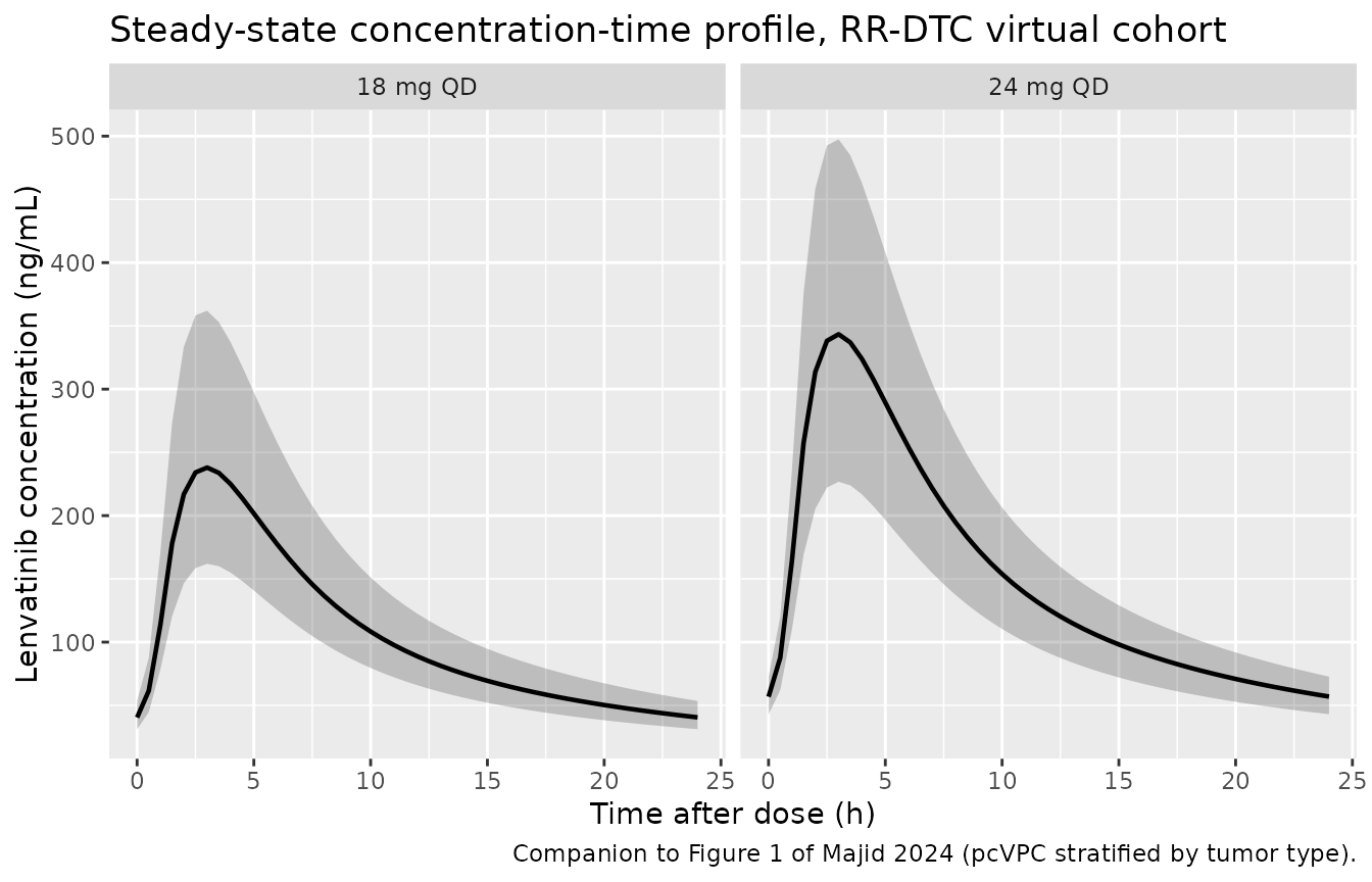

PKNCA validation

The paper publishes no NCA table, so the reference used here is the paper’s own supplement-published exposure formula. Text S1 derives the daily AUC that is carried into both PK/PD models as

AUC = 1000 * F1 * DGRP / CL

i.e. 1000 x relative bioavailability x daily dose (mg) / individual apparent clearance (L/h). At steady state this must equal the NCA AUC over one dosing interval, so it is an exact per-subject answer key for the PK model and simultaneously validates the definition of the AUC_LEN covariate that the two PD models consume.

pk_nca_in <- pk_sim |>
  filter(!is.na(Cc)) |>
  select(id, time, Cc, treatment)

conc_obj <- PKNCA::PKNCAconc(pk_nca_in, Cc ~ time | treatment + id,
                             concu = "ng/mL", timeu = "h")
dose_obj <- PKNCA::PKNCAdose(
  pk_events |> filter(evid == 1) |> select(id, time, amt, treatment),
  amt ~ time | treatment + id, doseu = "mg"
)

intervals <- data.frame(
  start = last_dose, end = last_dose + tau,
  cmax = TRUE, tmax = TRUE, cmin = TRUE, auclast = TRUE, cav = TRUE
)
nca_res <- PKNCA::pk.nca(PKNCA::PKNCAdata(conc_obj, dose_obj, intervals = intervals))

# Per-subject answer key (Text S1). Testing per subject rather than on group
# medians is deliberate: a median comparison hides per-subject error.
key <- pk_events |>
  distinct(id, WT, treatment, dose_mg) |>
  mutate(cl_ind = 6.28 * 0.951 * (WT / 73.2)^0.75,
         auclast = 1000 * 0.882 * dose_mg / cl_ind)

identity_check <- as.data.frame(nca_res) |>
  filter(PPTESTCD == "auclast") |>
  select(id, treatment, simulated = PPORRES) |>
  left_join(key |> select(id, reference = auclast), by = "id") |>
  mutate(pct_diff = (simulated - reference) / reference * 100)

stopifnot(max(abs(identity_check$pct_diff)) < 0.5)

identity_check |>
  group_by(treatment) |>
  summarise(`Max |% diff|` = max(abs(pct_diff)),
            `Median % diff` = median(pct_diff), .groups = "drop") |>
  knitr::kable(digits = 4,
               caption = "Per-subject steady-state AUC0-tau versus the Text S1 formula 1000 * F1 * Dose / CL.")

Per-subject steady-state AUC0-tau versus the Text S1 formula 1000 * F1 * Dose / CL.
treatment	Max \|% diff\|	Median % diff
18 mg QD	0.3816	-0.1993
24 mg QD	0.3687	-0.1819

published <- key |>
  group_by(treatment) |>
  summarise(auclast = median(auclast), .groups = "drop")

cmp <- nlmixr2lib::ncaComparisonTable(
  simulated = nca_res,
  reference = published,
  by = "treatment",
  params = "auclast",
  units = c(auclast = "ng*h/mL"),
  tolerance_pct = 20
)
knitr::kable(cmp, caption = "Simulated steady-state AUC0-tau versus the Text S1 model-derived exposure. * differs by >20%.")

Simulated steady-state AUC0-tau versus the Text S1 model-derived exposure. * differs by >20%.
NCA parameter	treatment	Reference	Simulated	% diff
AUClast (ng*h/mL)	18 mg QD	2570	2570	-0.2%
AUClast (ng*h/mL)	24 mg QD	3670	3670	-0.2%

The reference AUC values (2658 and 3544 ng*h/mL for the typical 73.2 kg DTC patient at 18 and 24 mg) also set the exposure levels used throughout the PD sections below.

cl_typ <- 6.28 * 0.951                       # DTC patient at the 73.2 kg reference weight
auc_of <- function(dose) 1000 * 0.882 * dose / cl_typ
auc_18 <- auc_of(18); auc_24 <- auc_of(24)
c(`18 mg` = auc_18, `24 mg` = auc_24)
#>    18 mg    24 mg 
#> 2658.281 3544.375

Serum biomarker PK/PD

Four turnover pools share one Emax, one EC50 and one disease-progression slope; baseline, mean residence time and Hill coefficient are per-biomarker. Lenvatinib inhibits Kout for VEGF and FGF-23 (levels rise) and Kin for Tie-2 and Ang-2 (levels fall). The models carry no dosing events: exposure enters as the AUC_LEN covariate.

sim_biomarkers <- function(dose_label, auc) {
  ev <- as.data.frame(rxode2::et(seq(0, 52 * 7 * 24, by = 6)))  # hours, 52 weeks
  ev$id <- 1L
  ev$AUC_LEN <- auc
  rxode2::rxSolve(rxode2::zeroRe(mod_bm), ev, omega = NA, sigma = NA) |>
    as.data.frame() |>
    mutate(week = time / 24 / 7, treatment = dose_label)
}

bm_sim <- bind_rows(sim_biomarkers("18 mg QD", auc_18),
                    sim_biomarkers("24 mg QD", auc_24))

bm_baseline <- c(vegf = 0.370, tie2 = 14.6, ang2 = 3.36, fgf23 = 0.0990)

bm_long <- bm_sim |>
  select(week, treatment, all_of(names(bm_baseline))) |>
  pivot_longer(all_of(names(bm_baseline)), names_to = "biomarker", values_to = "value") |>
  mutate(baseline = bm_baseline[biomarker],
         pct_cfb = (value - baseline) / baseline * 100,
         biomarker = factor(biomarker, levels = c("vegf", "fgf23", "ang2", "tie2"),
                            labels = c("VEGF", "FGF-23", "Ang-2", "Tie-2")))

# Replicates the four serum-biomarker panels of Figure 4 of Majid 2024:
# model-predicted % change from baseline over 52 weeks at 18 and 24 mg QD.
ggplot(bm_long, aes(week, pct_cfb, colour = treatment)) +
  geom_hline(yintercept = 0, linetype = "dashed", colour = "grey50") +
  geom_line(linewidth = 0.8) +
  facet_wrap(~biomarker, scales = "free_y") +
  labs(x = "Time (weeks)", y = "Change from baseline (%)", colour = NULL,
       title = "Model-predicted serum biomarker time course, typical RR-DTC patient",
       caption = "Replicates the serum-biomarker panels of Figure 4 of Majid 2024.") +
  theme(legend.position = "bottom")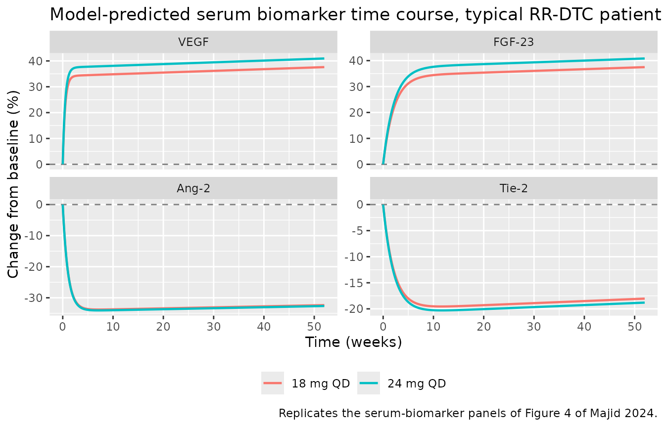

Validation against the Figure 4 narrative

Majid 2024 characterises Figure 4 qualitatively rather than numerically:

VEGF levels are predicted to increase faster than FGF-23 levels with a maximum increase achieved approximately after 2 weeks of treatment compared to approximately 8 weeks for FGF-23 […] Ang-2 levels are predicted to decrease faster than Tie-2 levels with a maximum decrease achieved approximately after 4 weeks of treatment, compared to approximately 8 weeks for Tie-2 […] followed by a gradual increase in both.

The “maximum” the authors read off the figure is the plateau of the drug-driven excursion, after which the linear disease-progression term makes every curve drift upward again. The corresponding model quantity is the time to reach 90% of the drug-driven extremum, tabulated below for the 24 mg arm.

timing <- bm_long |>
  filter(treatment == "24 mg QD") |>
  group_by(biomarker) |>
  summarise(
    extremum_pct = if (first(biomarker) %in% c("VEGF", "FGF-23")) max(pct_cfb) else min(pct_cfb),
    t90_week = week[which(abs(pct_cfb) >= 0.9 * abs(extremum_pct))[1]],
    .groups = "drop"
  ) |>
  mutate(paper_week = c(2, 8, 4, 8)[match(biomarker, c("VEGF", "FGF-23", "Ang-2", "Tie-2"))])

timing |>
  rename("Biomarker" = biomarker,
         "Extremum change from baseline (%)" = extremum_pct,
         "Time to 90% of extremum (weeks)" = t90_week,
         "Paper's stated time (weeks)" = paper_week) |>
  knitr::kable(digits = 2,
               caption = "Simulated time course versus the Figure 4 narrative of Majid 2024.")

Simulated time course versus the Figure 4 narrative of Majid 2024.
Biomarker	Extremum change from baseline (%)	Time to 90% of extremum (weeks)	Paper’s stated time (weeks)
VEGF	40.94	1.93	2
FGF-23	40.83	7.68	8
Ang-2	-34.06	2.36	4
Tie-2	-20.29	4.57	8

VEGF (1.9 vs “approximately 2” weeks) and FGF-23 (7.7 vs “approximately 8” weeks) reproduce the stated times closely. Ang-2 and Tie-2 plateau faster in the simulation than the figure text states, but the ordering the paper asserts – VEGF before FGF-23, Ang-2 before Tie-2 – holds, and both orderings follow directly from the mean residence times (VEGF 58.3 h < FGF-23 265 h; Ang-2 173 h < Tie-2 354 h).

stopifnot(
  timing$t90_week[timing$biomarker == "VEGF"]  < timing$t90_week[timing$biomarker == "FGF-23"],
  timing$t90_week[timing$biomarker == "Ang-2"] < timing$t90_week[timing$biomarker == "Tie-2"]
)

The paper also states that VEGF and FGF-23 rise while Ang-2 and Tie-2 fall, with a marginally larger excursion at 24 mg than at 18 mg – “suggestive of saturation of the pathway at these dose levels”, since both doses sit well above the common EC50 of 930 ng*h/mL.

direction <- bm_long |>
  group_by(treatment, biomarker) |>
  summarise(peak_excursion = pct_cfb[which.max(abs(pct_cfb))], .groups = "drop") |>
  pivot_wider(names_from = treatment, values_from = peak_excursion)

stopifnot(
  all(direction[[2]][direction$biomarker %in% c("VEGF", "FGF-23")] > 0),
  all(direction[[2]][direction$biomarker %in% c("Ang-2", "Tie-2")] < 0),
  all(abs(direction$`24 mg QD`) >= abs(direction$`18 mg QD`))
)
direction |>
  rename("Biomarker" = biomarker) |>
  knitr::kable(digits = 2,
               caption = "Peak excursion from baseline (%). Both doses exceed the common EC50 of 930 ng*h/mL, so the arms nearly coincide.")

Peak excursion from baseline (%). Both doses exceed the common EC50 of 930 ng*h/mL, so the arms nearly coincide.
Biomarker	18 mg QD	24 mg QD
VEGF	37.60	40.94
FGF-23	37.50	40.83
Ang-2	-33.78	-34.06
Tie-2	-19.55	-20.29

Tumor dynamics

The tumor-model fork

The deposited control stream (Supplementary Text S3) defines Tie-2-specific effect variables in its $PK block

IMAX1T =  IMAX2
IC50T  =  IC502/1000      ; IC50 for TIE2
HILLT  =  HILL2           ; Hill coefficient for TIE2 sigmoid Imax

and then never reads them. The $DES Tie-2 line instead picks up the VEGF-indexed input columns:

EFFT = IMAX1*(AUC+.1)**HILL /(IC50**HILL+(AUC+.1)**HILL)      ; TIE2

whereas the parallel Ang-2 line three rows below is written correctly with IMAX1A, HILLA and IC50A. Taking Text S3 literally has two consequences: the Hill coefficient becomes VEGF’s, fixed at 1 rather than Tie-2’s estimated 0.313; and IC50 is the common EC50 left on the ngh/mL scale (930) while the stream’s AUC has been rescaled to ugh/mL by AUC = LEVAVAUC/1000. The resulting 1000-fold mismatch drives the Tie-2 drug effect to 0.13% at the 24 mg steady-state exposure, i.e. the Tie-2 pool becomes drug-insensitive and its contribution to the tumor ODE is a pure disease-progression term.

The evidence points in two directions and the package therefore ships both readings rather than picking one:

Structural evidence favours the printed equations. Equation 2 gives Tie-2 its own Hill coefficient and EC50; Table 3’s abbreviation list defines KTie-2 as the “tumor size reduction rate constant for Tie-2”; and the paper’s headline finding is that Tie-2 is a statistically significant predictor of tumor response (154-point OFV drop with Tie-2 and Ang-2 added). Under the literal reading the Tie-2 term instead rises slightly over 52 weeks, so with a negative KTie-2 it contributes tumor growth, not reduction.
The paper’s only numeric tumor prediction favours the deposited stream. See the discriminator table below.

Majid_2024_lenvatinib_tumor implements the printed Equations 2 and 4; Majid_2024_lenvatinib_tumor_asdeposited transcribes Text S3 verbatim, including the (AUC+.1) numerical guard.

Simulation

The paper’s Results state: “For a typical 73.2 kg RR-DTC patient with a baseline tumor size of 70.2 mm the tumor shrinkage is predicted to be relatively faster and higher following 24 mg QD reaching over 35% following 52 weeks of treatment.”

Both tumor models emit some etas defaulted to non-mu referenced ... etaibase_prop, etaibase_add when compiled. That is expected and correct: those two unit-variance etas are consumed only inside the tumor(0) initial condition, where they push the observed baseline through the model’s own residual error (Text S3 $OMEGA slots 5 and 6, both 1 FIX). They are deliberately not mu-referenced, so the warning is suppressed in the chunks below.

sim_tumor <- function(mod, dose_label, auc, variant) {
  ev <- as.data.frame(rxode2::et(seq(0, 52, by = 0.25)))   # weeks
  ev$id <- 1L
  ev$AUC_LEN <- auc
  ev$TUM_SLD <- 70.2
  rxode2::rxSolve(rxode2::zeroRe(mod), ev, omega = NA, sigma = NA) |>
    as.data.frame() |>
    mutate(week = time, treatment = dose_label, variant = variant,
           pct_cfb = (tumor - 70.2) / 70.2 * 100,
           tie2_pct = (tie2 - 14.6) / 14.6 * 100,
           ang2_pct = (ang2 - 3.36) / 3.36 * 100)
}

tumor_sim <- bind_rows(
  sim_tumor(mod_tumA, "18 mg QD", auc_18, "A: printed Equations 2/4"),
  sim_tumor(mod_tumA, "24 mg QD", auc_24, "A: printed Equations 2/4"),
  sim_tumor(mod_tumB, "18 mg QD", auc_18, "B: Text S3 as deposited"),
  sim_tumor(mod_tumB, "24 mg QD", auc_24, "B: Text S3 as deposited")
)
#> ℹ parameter labels from comments will be replaced by 'label()'
#> ℹ parameter labels from comments will be replaced by 'label()'
#> ℹ parameter labels from comments will be replaced by 'label()'
#> ℹ parameter labels from comments will be replaced by 'label()'

# Replicates the tumor-size panel of Figure 4 of Majid 2024, drawn for both
# readings of the Tie-2 drug-effect line.
ggplot(tumor_sim, aes(week, pct_cfb, colour = treatment)) +
  geom_hline(yintercept = -35, linetype = "dotted", colour = "grey30") +
  geom_line(linewidth = 0.8) +
  facet_wrap(~variant) +
  labs(x = "Time (weeks)", y = "Tumor size change from baseline (%)", colour = NULL,
       title = "Model-predicted tumor dynamics, typical 73.2 kg RR-DTC patient",
       caption = paste("Replicates the tumor panel of Figure 4 of Majid 2024.",
                       "Dotted line: the paper's 'over 35%' claim for 24 mg at 52 weeks.")) +
  theme(legend.position = "bottom")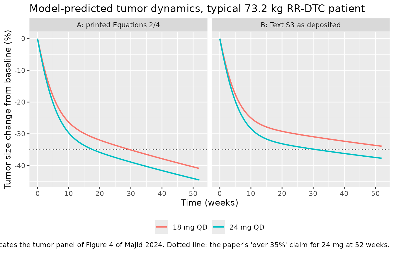

The discriminator

discriminator <- tumor_sim |>
  group_by(variant, treatment) |>
  summarise(`Tumor change at 52 weeks (%)` = pct_cfb[which.max(week)],
            `Tie-2 extremum (%)` = min(tie2_pct),
            `Ang-2 extremum (%)` = min(ang2_pct),
            .groups = "drop")

discriminator |>
  rename("Reading" = variant, "Dose" = treatment) |>
  knitr::kable(digits = 2,
               caption = "Both readings against the paper's 'over 35% at 52 weeks' claim for the 24 mg arm.")

Both readings against the paper’s ‘over 35% at 52 weeks’ claim for the 24 mg arm.
Reading	Dose	Tumor change at 52 weeks (%)	Tie-2 extremum (%)	Ang-2 extremum (%)
A: printed Equations 2/4	18 mg QD	-40.93	-19.55	-33.78
A: printed Equations 2/4	24 mg QD	-44.56	-20.29	-34.06
B: Text S3 as deposited	18 mg QD	-33.91	-0.03	-33.84
B: Text S3 as deposited	24 mg QD	-37.71	-0.05	-34.07

Reading B puts the 24 mg arm at -37.7% and the 18 mg arm at -33.9%, which makes “over 35%” a discriminating statement about the 24 mg arm – exactly the kind of sentence an author writes after reading the figure. Under reading A both arms clear 40%, so “over 35%” would be an oddly loose description of -44.6%. That single sentence is the strongest evidence that Figure 4 was generated by the control stream as written.

Against it: under reading B the Tie-2 pool never falls (its extremum is -0.05%, numerical noise) and ends 2.3% above baseline, so with KTie-2 negative the Tie-2 term contributes growth. That is incompatible with Equation 2, with Table 3’s legend, and with the paper’s conclusion that Tie-2 changes are associated with tumor response.

d <- discriminator
# Reading B reproduces the paper's "over 35%" claim as a discriminating statement.
stopifnot(
  d$`Tumor change at 52 weeks (%)`[d$variant == "B: Text S3 as deposited" &
                                     d$treatment == "24 mg QD"] < -35,
  d$`Tumor change at 52 weeks (%)`[d$variant == "B: Text S3 as deposited" &
                                     d$treatment == "18 mg QD"] > -35
)
# Reading B leaves Tie-2 drug-insensitive; reading A does not.
stopifnot(
  abs(d$`Tie-2 extremum (%)`[d$variant == "B: Text S3 as deposited"]) < 1,
  all(d$`Tie-2 extremum (%)`[d$variant == "A: printed Equations 2/4"] < -15)
)
# Both readings share an identical Ang-2 arm (the deposited Ang-2 line is correct).
stopifnot(
  max(abs(d$`Ang-2 extremum (%)`[d$variant == "A: printed Equations 2/4"] -
            d$`Ang-2 extremum (%)`[d$variant == "B: Text S3 as deposited"])) < 0.1
)

Sanity checks on the tumor ODE

rxode2 returns every intermediate of model() as an output column, so the individual terms of Equation 4 can be audited directly rather than re-derived.

# 1. Placebo. With no exposure the drug term vanishes and the biomarker pools
#    never move, so the tumor grows exponentially at KG = 0.00252 /week.
placebo <- sim_tumor(mod_tumA, "placebo", 0, "A: printed Equations 2/4")
#> ℹ parameter labels from comments will be replaced by 'label()'
observed_kg <- log(placebo$tumor[which.max(placebo$week)] / 70.2) / 52
stopifnot(abs(observed_kg - 0.00252) < 5e-4)

# 2. Resistance. DRV decays with lambda = 0.259 /week, so by 52 weeks the
#    drug-driven shrinkage term is numerically extinct.
a24 <- tumor_sim |> filter(variant == "A: printed Equations 2/4",
                           treatment == "24 mg QD")
drv_0  <- a24$drv[which.min(a24$week)]
drv_52 <- a24$drv[which.max(a24$week)]
stopifnot(drv_52 / drv_0 < 1e-4)

# 3. Yet the tumor is still shrinking at 52 weeks, because the two biomarker
#    terms together outweigh KG. This is the paper's mechanistic claim made
#    quantitative: late tumor control is carried by the Tie-2 / Ang-2 terms,
#    not by the exposure term.
late_rates <- function(variant_label) {
  x <- tumor_sim |>
    filter(variant == variant_label, treatment == "24 mg QD")
  x <- x[which.max(x$week), ]
  tibble(
    Reading = variant_label,
    `Growth KG` = x$kgrow,
    `Exposure term DRV` = x$drv,
    `Tie-2 term` = x$ktie2 * x$rel_tie2,
    `Ang-2 term` = x$kang2 * x$rel_ang2,
    `Net rate (/week)` = x$kgrow - (x$drv + x$ktie2 * x$rel_tie2 +
                                      x$kang2 * x$rel_ang2)
  )
}
rate_tbl <- bind_rows(late_rates("A: printed Equations 2/4"),
                      late_rates("B: Text S3 as deposited"))

stopifnot(
  # Under both readings the tumor is still shrinking at 52 weeks.
  all(rate_tbl$`Net rate (/week)` < 0),
  # Under A the Tie-2 term contributes shrinkage; under B it contributes growth.
  rate_tbl$`Tie-2 term`[rate_tbl$Reading == "A: printed Equations 2/4"] > 0,
  rate_tbl$`Tie-2 term`[rate_tbl$Reading == "B: Text S3 as deposited"] < 0
)

knitr::kable(rate_tbl, digits = 6,
             caption = paste("Terms of Equation 4 at week 52, 24 mg QD.",
                             "Positive Tie-2 / Ang-2 terms shrink the tumor;",
                             "a negative one grows it."))

Terms of Equation 4 at week 52, 24 mg QD. Positive Tie-2 / Ang-2 terms shrink the tumor; a negative one grows it.
Reading	Growth KG	Exposure term DRV	Tie-2 term	Ang-2 term	Net rate (/week)
A: printed Equations 2/4	0.00252	0	0.002106	0.004700	-0.004286
B: Text S3 as deposited	0.00252	0	-0.000260	0.004702	-0.001922

Placebo growth reproduces KG to 0.00283 /week against the published 0.00252, and the exposure term has fallen to 4.9^{-6} of its week-0 value. The last row is the sign-level statement of the fork: under the printed equations the Tie-2 term shrinks the tumor, while under the deposited stream it grows it, because the drug-insensitive Tie-2 pool drifts above baseline on the disease-progression slope and KTie-2 is negative.

Between-subject variability

The tumor model carries additive IIV on KG, Emax and lambda, exponential IIV on EC50 and KAng-2, and unit-variance etas that push the observed baseline through the model’s own residual error into the initial condition.

set.seed(20240614)
n_vpc <- 100L
vpc_events <- bind_rows(
  tibble(id = seq_len(n_vpc),          AUC_LEN = auc_18, treatment = "18 mg QD"),
  tibble(id = n_vpc + seq_len(n_vpc),  AUC_LEN = auc_24, treatment = "24 mg QD")
) |>
  mutate(TUM_SLD = 70.2) |>
  tidyr::crossing(time = seq(0, 52, by = 1)) |>
  mutate(evid = 0L, amt = NA_real_, cmt = "tumor")

vpc <- rxode2::rxSolve(mod_tumA, events = vpc_events, keep = "treatment") |>
  as.data.frame() |>
  mutate(pct_cfb = (tumor - 70.2) / 70.2 * 100)
#> ℹ parameter labels from comments will be replaced by 'label()'

stopifnot(length(unique(vpc$id)) == 2L * n_vpc)

vpc |>
  group_by(treatment, time) |>
  summarise(Q05 = quantile(pct_cfb, 0.05), Q50 = median(pct_cfb),
            Q95 = quantile(pct_cfb, 0.95), .groups = "drop") |>
  ggplot(aes(time, Q50)) +
  geom_ribbon(aes(ymin = Q05, ymax = Q95), alpha = 0.25) +
  geom_line(linewidth = 0.8) +
  facet_wrap(~treatment) +
  labs(x = "Time (weeks)", y = "Tumor size change from baseline (%)",
       title = "Tumor-size VPC, reading A (printed Equations 2 and 4)",
       caption = "Companion to Figure 3 of Majid 2024 (pcVPC of tumor size, stratified by study).")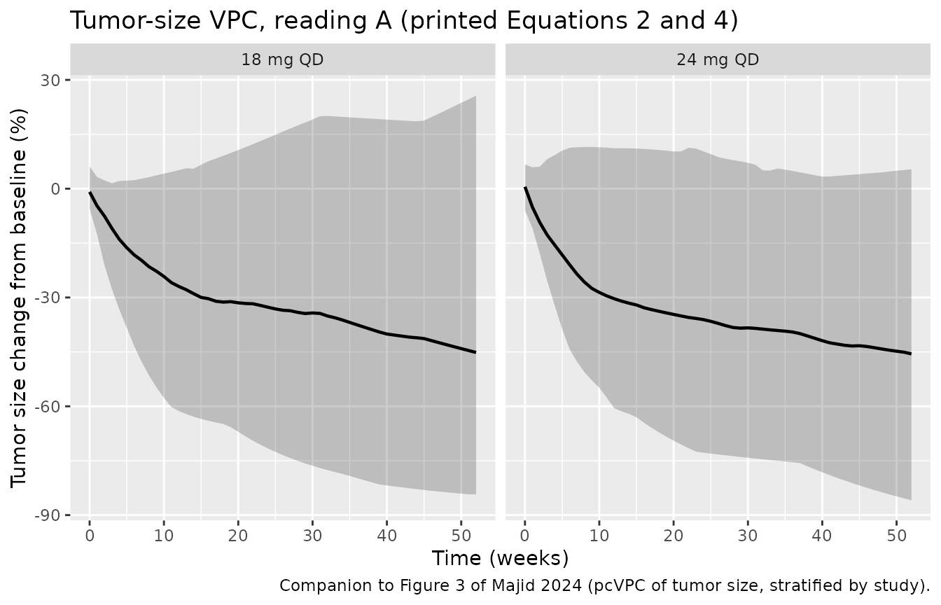

Assumptions and deviations

The Tie-2 fork (Errata)

The deposited Tie-2 drug-effect line in Text S3 uses the VEGF-indexed effect columns and leaves its EC50 on a 1000-fold mismatched unit scale, contradicting the paper’s printed Equations 2 and 4 and its Table 3 legend. Because the structural evidence and the paper’s single numeric tumor prediction point in opposite directions, both readings ship: Majid_2024_lenvatinib_tumor (printed equations) and Majid_2024_lenvatinib_tumor_asdeposited (Text S3 verbatim). Table 3’s parameter estimates were produced by whichever stream was actually run, so this is a substantive fork, not a cosmetic one. Users reproducing published Figure 4 numbers should prefer the as-deposited variant; users wanting the model the paper describes should prefer the other.

Unit labels

Table 2 prints the biomarker baselines as ng/L, Table S2 prints Tie-2 as ug/mL, and the Methods “Model-based PK/PD simulations” paragraph prints all four as ng/mL. The Methods bioanalysis detection ranges (Ang-2 0.188-64 ng/mL, Tie-2 3.10-200 ng/mL, VEGF 31-4000 pg/mL) bracket the reported baselines only on the ng/mL scale, so ng/mL is used throughout. FGF-23’s printed range of “20-150 ng/mL” is itself almost certainly a pg/mL typo: the Kainos CY-4000 intact-FGF23 kit is a pg/mL assay, and the 0.100 ng/mL baseline (= 100 pg/mL) sits inside 20-150 pg/mL.

The `(AUC+.1)` numerical guard

Both PD control streams write (AUC+.1) inside the sigmoid. In the biomarker stream AUC is in ngh/mL, so the guard is 0.1 ngh/mL – negligible against an EC50 of 930. In the tumor stream AUC has been rescaled to ugh/mL, so the same literal* 0.1 becomes 100 ngh/mL of pseudo-exposure. It is dropped from Majid_2024_lenvatinib_biomarkers and Majid_2024_lenvatinib_tumor (the printed Equations 1-2 carry no guard, and under reading A the guard would produce 11.4% Tie-2 inhibition at zero exposure, contradicting the paper’s statement that placebo patients follow the disease-progression model alone). It is retained* in Majid_2024_lenvatinib_tumor_asdeposited, where literal fidelity is the point and where the mismatched EC50 renders it numerically inert (~4e-5 of inhibition at zero exposure).

IIV scale

Tables 1, 2 and 3 print IIV under a “CV%” header whose footnote defines it as “square root of variance x 100” – i.e. omega x 100 on the log scale, not a linear-space coefficient of variation. Variances are therefore entered as (CV%/100)^2 with no log-normal back-conversion. Every $OMEGA initial estimate in Texts S1-S3 is a variance on the same scale and corroborates this reading (e.g. D1 init 1.0 vs final 0.967^2 = 0.935; VEGF MRT init 2.5 vs 1.54^2 = 2.37). Note that the predecessor model Gupta_2016_lenvatinib quotes the same footnote and then applies the log-normal conversion anyway; that is a pre-existing inconsistency in the library, not a change introduced here.

PK residual error

Text S1 implements three mutually exclusive residual-error branches selected by study type and time after dose (healthy-subject studies 17.6% proportional; patient studies 37.5% proportional; time after dose <= 2 h 42.9% proportional plus 20.5 ng/mL additive). nlmixr2 has no covariate-conditional residual-error construct, so the packaged model carries the patient-study proportional arm – the branch that applies to the RR-DTC cohort the two PD models are built on.

Absorption structure

The paper’s prose calls the absorption “simultaneous first- and zero-order”. Text S1 settles what that means: $SUBROUTINES ADVAN12 TRANS4 with a single dosing compartment, a single F1, and D1 defined for compartment 1 (the depot). The absorption is therefore sequential – zero-order into the depot over D1, then first-order at ka out of it – with no parallel dose split. The predecessor Gupta_2016_lenvatinib had to assume a 50:50 parallel split and flags that assumption in its own comments; this supplement resolves it.

Other simplifications

The sequential fit is reproduced as a sequential fit. The biomarker and tumor models take lenvatinib exposure as the AUC_LEN data column rather than solving the PK ODE, exactly as Texts S2 and S3 do. Compute AUC_LEN from the PK model with the Text S1 formula validated above.
The tumor model fixes its carried Tie-2 / Ang-2 turnover parameters at the biomarker model’s typical values. In the source they arrive as per-subject empirical Bayes estimates in the input data, which a packaged model cannot carry; users refitting should supply them per subject.
Text S3 integrates two additional “untreated” reference states for Tie-2 and Ang-2 that are never read by the tumor ODE or the $ERROR block. They are omitted from both tumor model files.
Concomitant CYP3A4 inducers appear in the Gupta 2016 predecessor but not in the Majid 2024 final model (only 6 of 1921 subjects were exposed); no inducer term is carried.
The ALP upper limit of normal is taken as 120 U/L, a representative adult value matching the choice in Gupta_2016_lenvatinib. Text S1 codes the covariate from an ALP/ULN ratio column, so users with their own laboratory ULN should scale the threshold accordingly.
The virtual cohorts here are illustrative: body weight is drawn log-normally around the published median, and albumin, ALP, tumor type and formulation are held at the RR-DTC modal values rather than resampled from Table S2’s joint distribution.
No thyroglobulin or TSH model is provided; the authors did not develop one, citing extreme variability in those biomarkers.

Model and source

Population

Source trace

Population PK

Virtual cohort

Simulation

PKNCA validation

Serum biomarker PK/PD

Validation against the Figure 4 narrative

Tumor dynamics

The tumor-model fork

Simulation

The discriminator

Sanity checks on the tumor ODE

Between-subject variability

Assumptions and deviations

The Tie-2 fork (Errata)

Unit labels

The (AUC+.1) numerical guard

IIV scale

PK residual error

Absorption structure

Other simplifications

The `(AUC+.1)` numerical guard