Cafedrine/theodrenaline vs ephedrine: maternal haemodynamics and neonatal acidosis (Dings 2026)

Model and source

This paper contributes two model files, mirroring its own two-part structure (Appendix A.1 maternal haemodynamics, Appendix A.2 newborn outcomes):

• Dings_2026_cafedrine_theodrenaline_ephedrine – the maternal haemodynamic population K/PD model (ODE-based, fitted in NONMEM 7.4.3 with FOCE-I).
• Dings_2026_neonatal_acidosis – the three stepwise linear regressions for the newborn umbilical-arterial biomarkers (fitted in R with mixlm).

They are coupled: two of the base-excess predictors are per-subject parameters of the maternal model, and the strongest predictor of both pH and base excess is derived from the maternal model’s simulated MAP-time profile. This vignette walks the paper as one unit and exercises both files together.

• Citation: Dings C, Lehr T, Kranke P, Vojnar B, Gaik C, Koch T, Eberhart L, Huljic-Lankinen S, Murst M, Kreuer S. Pharmacometric Analysis of Cafedrine/Theodrenaline Versus Ephedrine on Maternal Hemodynamics and Neonatal Acidosis During Cesarean Section. Pharmaceutics. 2026;18(3):296. doi:10.3390/pharmaceutics18030296
• Article: https://doi.org/10.3390/pharmaceutics18030296
• Parent study (HYPOTENS design): https://doi.org/10.1080/03007995.2018.1483227
• Parent study (primary results): https://doi.org/10.1097/EJA.0000000000001590

mat <- rxode2::rxode(readModelDb("Dings_2026_cafedrine_theodrenaline_ephedrine"))
#> ℹ parameter labels from comments will be replaced by 'label()'
neo <- rxode2::rxode(readModelDb("Dings_2026_neonatal_acidosis"))

Population

The HYPOTENS study was a prospective, open-label, two-armed, non-interventional study run at multiple German centres between July 2016 and February 2018 (Dings 2026 Section 2.1). Parturients undergoing elective caesarean section under spinal anaesthesia who developed hypotension (SBP < 100 mmHg or < 90% of the pre-operative baseline SBP) were treated at the attending anaesthesiologist’s discretion with intravenous boluses of either cafedrine/theodrenaline (C/T, a 20:1 fixed combination; doses expressed as cafedrine equivalents) or ephedrine. Patients given prophylactic antihypotensive treatment were excluded.

Of 283 per-protocol patients, 40 (14.1%) were excluded for blood loss > 1000 mL, colloid or blood-product administration, conversion to general anaesthesia, or a local anaesthetic other than bupivacaine, leaving 243 parturients: 135 (55.6%) C/T and 108 (44.4%) ephedrine (Section 3.1).

pop <- rxode2::rxode(readModelDb("Dings_2026_cafedrine_theodrenaline_ephedrine"))$meta$population
#> ℹ parameter labels from comments will be replaced by 'label()'
tibble::tibble(Field = names(pop), Value = vapply(pop, function(x) paste(as.character(x), collapse = "; "), character(1))) |>
  knitr::kable()

Field	Value
species	human
n_subjects	243
n_studies	1
age_range	NA
age_median	33.4 years (mean; SD 5.22)
weight_range	NA
weight_median	87.6 kg (mean; SD 19.7)
sex_female_pct	100
race_ethnicity	Not reported in Dings 2026; multicentre German cohort.
disease_state	Spinal-anaesthesia-induced hypotension (SBP < 100 mmHg or < 90% of the pre-operative baseline SBP) during elective caesarean section in parturients at term. Prophylactically treated patients were excluded.
dose_range	Intravenous boluses at the attending anaesthesiologist’s discretion. Cafedrine/theodrenaline 10-200 mg per dose (most common single dose 50 mg; median cumulative dose over 30 min 100 mg, range 20-400 mg), expressed as cafedrine equivalents. Ephedrine 5-40 mg per dose (most common 15 mg; median cumulative 30 mg, range 10-120 mg).
regions	Germany (multicentre)
notes	HYPOTENS study (Eberhart 2018, Curr Med Res Opin 34:953-961; primary results Kranke 2021, Eur J Anaesthesiol 38:1067-1076), a prospective, open-label, two-armed, non-interventional study conducted July 2016 - February 2018. Of 283 per-protocol patients, 40 (14.1%) were excluded for blood loss > 1000 mL, colloid / blood-product administration, conversion to general anaesthesia, or a local anaesthetic other than bupivacaine, leaving 243 analysed: 135 (55.6%) cafedrine/theodrenaline and 108 (44.4%) ephedrine. Haemodynamics were recorded immediately before the first bolus and at 1-10, 12, 15, 20, 25 and 30 min after it. Demographics from Dings 2026 Tables 1 and 2. NOTE: no pharmacokinetic samples were obtained, so every kinetic parameter here is a functional descriptor of the response time course, NOT a systemic pharmacokinetic quantity.

Maternal haemodynamics were recorded immediately before the first antihypotensive bolus and at 1-10, 12, 15, 20, 25 and 30 min after it. Two pre-treatment anchors are used throughout and the distinction is load-bearing: pre-surgery is the last value before anaesthesia, baseline is the value at hypotension diagnosis.

tibble::tribble(
  ~Parameter,                                        ~`C/T (n = 135)`, ~`Ephedrine (n = 108)`,
  "Pre-surgery MAP (mmHg)",                          "101 (13.9)",     "101 (14.2)",
  "Pre-surgery SBP (mmHg)",                          "139 (18.6)",     "138 (18.3)",
  "Pre-surgery HR (beats/min)",                      "92.6 (14.9)",    "91.7 (15.3)",
  "Baseline MAP (mmHg)",                             "64.2 (13.5)",    "64.5 (9.87)",
  "Baseline SBP (mmHg)",                             "92.3 (15.6)",    "93.0 (12.8)",
  "Baseline HR (beats/min)",                         "85.4 (22.1)",    "87.5 (22.1)",
  "Duration of MAP < pre-surgery MAP (min)",         "10.1 (6.16)",    "10.2 (5.76)",
  "Bupivacaine amount (mg)",                         "10.5 (2.44)",    "10.2 (1.95)",
  "Spinal block height (thoracic segment)",          "5.79 (1.93)",    "5.02 (1.22)",
  "Cord clamping to blood sampling (min)",           "7.81 (6.64)",    "4.65 (5.44)",
  "Umbilical arterial pH",                           "7.32 (0.051)",   "7.31 (0.070)",
  "Umbilical arterial base excess (mmol/L)",         "-0.933 (2.1)",   "-1.94 (2.38)",
  "Umbilical arterial lactate (mg/dL)",              "18.3 (6.83)",    "24.7 (13.9)"
) |>
  knitr::kable(caption = "Dings 2026 Table 2, mean (SD). Reproduced for reference; used below as validation targets.")

Dings 2026 Table 2, mean (SD). Reproduced for reference; used below as validation targets.

Parameter	C/T (n = 135)	Ephedrine (n = 108)
Pre-surgery MAP (mmHg)	101 (13.9)	101 (14.2)
Pre-surgery SBP (mmHg)	139 (18.6)	138 (18.3)
Pre-surgery HR (beats/min)	92.6 (14.9)	91.7 (15.3)
Baseline MAP (mmHg)	64.2 (13.5)	64.5 (9.87)
Baseline SBP (mmHg)	92.3 (15.6)	93.0 (12.8)
Baseline HR (beats/min)	85.4 (22.1)	87.5 (22.1)
Duration of MAP < pre-surgery MAP (min)	10.1 (6.16)	10.2 (5.76)
Bupivacaine amount (mg)	10.5 (2.44)	10.2 (1.95)
Spinal block height (thoracic segment)	5.79 (1.93)	5.02 (1.22)
Cord clamping to blood sampling (min)	7.81 (6.64)	4.65 (5.44)
Umbilical arterial pH	7.32 (0.051)	7.31 (0.070)
Umbilical arterial base excess (mmol/L)	-0.933 (2.1)	-1.94 (2.38)
Umbilical arterial lactate (mg/dL)	18.3 (6.83)	24.7 (13.9)

Model structure

No pharmacokinetic samples were taken (Section 2.1), and no published PK model exists for cafedrine, theodrenaline or ephedrine. The authors therefore used a K/PD approach: exposure is a virtual one-compartment kinetic model with first-order elimination, with the apparent volume fixed to 1 L purely for identifiability (Section 2.2). Every kinetic parameter here is a functional descriptor of the response time course, not a systemic pharmacokinetic quantity – a caveat the paper’s Discussion states repeatedly.

The K/PD concentration then feeds two parallel first-order lag cascades of different speed, whose terminal stages sum to a single driver concentration:

• a slow chain of 3 stages at ktr_slow = 0.107/min (mean transit time 28.0 min) carrying the persistence of the response, and
• a fast chain of 4 stages at ktr_fast = 1.76/min (mean transit time 2.27 min) carrying its onset.

That driver acts through three parallel Emax relationships on heart rate, mean arterial pressure and systolic blood pressure, each anchored on the subject’s own at-diagnosis baseline. A separate decaying state carries the progressive blood-pressure fall of the spinal anaesthetic itself, and step effects capture surgical incision and uterotomy.

Source trace

Every equation and every ini() value, with its source location.

tibble::tribble(
  ~Component, ~`Source location`, ~Notes,
  "d/dt(depot_kpd) = -kel * depot_kpd",                    "Eq. A1",  "Virtual K/PD compartment, IV bolus; kel = CL/V",
  "Slow cascade, 3 stages at ktr_slow",                    "Eqs A2-A4", "Sign corrected; see Errata item 1",
  "Fast cascade, 4 stages at ktr_fast",                    "Eqs A5-A8", "Sign corrected; see Errata item 1",
  "d/dt(effect_anaesthesia) = -kdel * effect_anaesthesia", "Eq. A9",  "Unit amount dosed at anaesthesia",
  "conc = effect_slow3 + effect_fast4",                    "Eq. A10", "Printed as A4 + A9; see Errata item 2",
  "anaes_eff = exp(-kdel*T_ANAESTHESIA) - effect_anaesthesia", "Eq. A11", "Rises from 0 at t = 0",
  "hr  = HR_BL  + (rmax_hr - HR_BL)*conc/(conc+ec50_hr) + eff_event_hr*iu",  "Eq. A12", "Emax on the subject's own baseline",
  "map = MAP_BL + (rmax_map - MAP_BL)*conc/(conc+ec50_map) + eff_bp*anaes_eff + eff_event_pp/3*iu", "Eq. A13", "MAP receives one third of the pulse-pressure step",
  "sbp = SBP_BL + (rmax_sbp - SBP_BL)*conc/(conc+ec50_sbp) + eff_bp*anaes_eff + eff_event_pp*iu",   "Eq. A14", "SBP receives the full pulse-pressure step",
  "Continuous covariates: (COV/median)^theta",             "Eq. 1",   "Centred at the population median",
  "Categorical covariates: 1 + COV*theta",                 "Eq. 2",   "Fractional change vs reference"
) |>
  knitr::kable(caption = "Maternal haemodynamic model equations (Dings 2026 Appendix A.1).")

Maternal haemodynamic model equations (Dings 2026 Appendix A.1).

Component	Source location	Notes
d/dt(depot_kpd) = -kel * depot_kpd	Eq. A1	Virtual K/PD compartment, IV bolus; kel = CL/V
Slow cascade, 3 stages at ktr_slow	Eqs A2-A4	Sign corrected; see Errata item 1
Fast cascade, 4 stages at ktr_fast	Eqs A5-A8	Sign corrected; see Errata item 1
d/dt(effect_anaesthesia) = -kdel * effect_anaesthesia	Eq. A9	Unit amount dosed at anaesthesia
conc = effect_slow3 + effect_fast4	Eq. A10	Printed as A4 + A9; see Errata item 2
anaes_eff = exp(-kdel*T_ANAESTHESIA) - effect_anaesthesia	Eq. A11	Rises from 0 at t = 0
hr = HR_BL + (rmax_hr - HR_BL)conc/(conc+ec50_hr) + eff_event_hriu	Eq. A12	Emax on the subject’s own baseline
map = MAP_BL + (rmax_map - MAP_BL)conc/(conc+ec50_map) + eff_bpanaes_eff + eff_event_pp/3*iu	Eq. A13	MAP receives one third of the pulse-pressure step
sbp = SBP_BL + (rmax_sbp - SBP_BL)conc/(conc+ec50_sbp) + eff_bpanaes_eff + eff_event_pp*iu	Eq. A14	SBP receives the full pulse-pressure step
Continuous covariates: (COV/median)^theta	Eq. 1	Centred at the population median
Categorical covariates: 1 + COV*theta	Eq. 2	Fractional change vs reference

mat$iniDf |>
  dplyr::filter(is.na(neta1) | neta1 == neta2) |>
  dplyr::transmute(
    Parameter = name,
    Estimate = signif(est, 6),
    Fixed = ifelse(!is.na(fix) & fix, "yes", ""),
    Label = ifelse(is.na(label), "", label)
  ) |>
  dplyr::rename("Fixed?" = Fixed) |>
  knitr::kable(caption = "Maternal model ini() values. Every row traces to Dings 2026 Table A1; the per-row source and RSE are in the in-file comments of the model file.")

Maternal model ini() values. Every row traces to Dings 2026 Table A1; the per-row source and RSE are in the in-file comments of the model file.

Parameter	Estimate	Fixed?	Label
lcl	-2.3320100		K/PD clearance (L/min)
lvc	0.0000000	yes	K/PD apparent volume of distribution (L)
lktr_slow	-2.2349300		Transit rate of the slow (long-term) effect cascade (1/min)
lktr_fast	0.5653140		Transit rate of the fast (short-term) effect cascade (1/min)
lrmax_hr	4.3541400		Maximum attainable heart rate (beats/min)
lrmax_map	4.7791200		Maximum attainable mean arterial pressure (mmHg)
lrmax_sbp	5.1299000		Maximum attainable systolic blood pressure (mmHg)
lec50_hr	1.7281100		Driver concentration for half-maximal heart-rate effect (mg/L)
lec50_map	4.1222800		Driver concentration for half-maximal MAP effect (mg/L)
lec50_sbp	4.1651100		Driver concentration for half-maximal SBP effect (mg/L)
lkdel	-1.7660900		Rate constant of the anaesthesia blood-pressure effect (1/min)
eff_anaes_bp	-9.7800000		Anaesthesia effect on MAP and SBP at a T5 block (mmHg)
eff_event_hr	2.7500000		Incision / uterotomy effect on heart rate, per event (beats/min)
eff_event_pp	2.3900000		Incision / uterotomy effect on pulse pressure, per event (mmHg)
e_bmi_cl	-0.9480000		Power exponent of BMI on K/PD clearance, centred at 30 kg/m^2
e_dbp_bl_vc	-1.4900000		Power exponent of baseline DBP on K/PD volume, centred at 50 mmHg
e_hr_presurg_rmax_hr	0.3990000		Power exponent of pre-surgery HR on the HR ceiling, centred at 92 beats/min
e_map_presurg_rmax_map	0.4990000		Power exponent of pre-surgery MAP on the MAP ceiling, centred at 100 mmHg
e_map_bl_rmax_map	-0.5300000		Power exponent of baseline MAP on the MAP ceiling, centred at 64 mmHg
e_sbp_presurg_rmax_sbp	0.5770000		Power exponent of pre-surgery SBP on the SBP ceiling, centred at 139 mmHg
e_sbp_bl_rmax_sbp	-0.4940000		Power exponent of baseline SBP on the SBP ceiling, centred at 92 mmHg
e_spinal_block_effbp	-2.0500000		Power exponent of spinal block segment number on the anaesthesia BP effect, centred at T5
e_trt_ephedrine_rmax_hr	0.1500000		Fractional change in the HR ceiling for ephedrine vs cafedrine/theodrenaline
e_trt_ephedrine_ec50	-0.7110000		Fractional change in ALL THREE EC50 values for ephedrine vs cafedrine/theodrenaline
propSd_hr	0.1300000		Proportional residual SD for heart rate
propSd_map	0.0937000		Proportional residual SD for MAP
propSd_sbp	0.0855000		Proportional residual SD for SBP
etalcl	0.3698800		Table A1 Clearance IIV 66.9 %CV, RSE 9.15%
etalvc	0.4703940		Table A1 Volume IIV 77.5 %CV, RSE 13%
etalktr_fast	0.3903390		Table A1 Ktr2 IIV 69.1 %CV, RSE 5.77%
etalrmax_hr	0.0246575		Table A1 MAXHR IIV 15.8 %CV, RSE 7.35%
etalrmax_map	0.0268610		Table A1 MAXMAP IIV 16.5 %CV, RSE 15.4%
etalrmax_sbp	0.0172739		Table A1 MAXSBP IIV 13.2 %CV, RSE 18.2%

neo$iniDf |>
  dplyr::transmute(Parameter = name, Estimate = signif(est, 6),
                   Label = ifelse(is.na(label), "", label)) |>
  knitr::kable(caption = "Neonatal regression ini() values: intercepts and slopes from Dings 2026 Tables A2 (pH), A3 (base excess) and A4 (lactate).")

Neonatal regression ini() values: intercepts and slopes from Dings 2026 Tables A2 (pH), A3 (base excess) and A4 (lactate).

Parameter	Estimate	Label
ph_ua_int	7.520000	Umbilical-arterial pH intercept
e_dur_map_below_presurg_ph	-0.001770	pH change per minute of maternal MAP below pre-surgery MAP
e_ega_ph	-0.000822	pH change per additional day of pregnancy duration
e_spinal_block_ph	0.005340	pH change per additional spinal segment number
be_ua_int	-2.090000	Umbilical-arterial base excess intercept (mmol/L)
e_trt_cafedrine_theodrenaline_be	3.260000	Base-excess change for maternal C/T vs untreated (mmol/L)
e_trt_ephedrine_be	2.640000	Base-excess change for maternal ephedrine vs untreated (mmol/L)
e_dur_map_below_presurg_be	-0.105000	Base-excess change per minute of maternal MAP below pre-surgery MAP (mmol/L/min)
e_spinal_block_be	0.300000	Base-excess change per additional spinal segment number (mmol/L)
e_dose_bupivacaine_mg_be	-0.186000	Base-excess change per mg maternal bupivacaine (mmol/L/mg)
e_wt_be	0.017600	Base-excess change per kg maternal body weight (mmol/L/kg)
e_maxhr_kpd_be	-0.025600	Base-excess change per beat/min of the maternal K/PD MAXHR (mmol/L/bpm)
e_kel_kpd_be	-1.740000	Base-excess change per 1/min of the maternal K/PD kel (mmol/L per 1/min)
lactate_ua_int	3.430000	Umbilical-arterial lactate intercept (mg/dL)
e_t_cordclamp_sampling_lactate	0.708000	Lactate change per minute from cord clamping to sampling (mg/dL/min)
e_trt_ephedrine_lactate	5.460000	Lactate change for maternal ephedrine vs C/T or untreated (mg/dL)
e_dose_bupivacaine_mg_lactate	1.050000	Lactate change per mg maternal bupivacaine (mg/dL/mg)
addSd_ph_ua	0.000000	Additive residual SD for umbilical-arterial pH (not reported in the source)
addSd_be_ua	0.000000	Additive residual SD for umbilical-arterial base excess (not reported in the source)
addSd_lactate_ua	0.000000	Additive residual SD for umbilical-arterial lactate (not reported in the source)

Why there is no PKNCA section

NCA is not applicable and is deliberately omitted. No drug concentrations were ever measured; the only “concentration” in the model is the virtual K/PD state whose volume was fixed to 1 L as a scaling device. An AUC or Cmax computed from it would be a reparameterisation of the dose, not a pharmacokinetic quantity, and reporting one would imply an exposure metric the study cannot support. The model is instead validated below against the paper’s own published derived quantities, typical-value simulations and cohort results.

Validation 1: analytic anchors

Section 3.2 reports several quantities that are exact algebraic consequences of Table A1, so they gate the transcription directly.

ini <- setNames(mat$iniDf$est, mat$iniDf$name)
cl <- exp(ini[["lcl"]]); vc <- exp(ini[["lvc"]]); kel <- cl / vc
anchors <- tibble::tibble(
  Quantity = c("Effect half-life (min)", "Slow-chain mean transit time (min)",
               "Fast-chain mean transit time (min)", "Ephedrine MAP EC50 (mg/L)",
               "Ephedrine SBP EC50 (mg/L)", "Ephedrine HR EC50 (mg/L)",
               "Ephedrine MAXHR (beats/min)", "MAP step / SBP step at incision"),
  Reproduced = c(
    log(2) / kel,
    3 / exp(ini[["lktr_slow"]]),
    4 / exp(ini[["lktr_fast"]]),
    # Section 3.2 quotes the ephedrine EC50s computed from its own rounded C/T
    # values (61.4 / 64 / 5.6), so reproduce them on the same basis.
    61.4 * (1 + ini[["e_trt_ephedrine_ec50"]]),
    64.0 * (1 + ini[["e_trt_ephedrine_ec50"]]),
    5.6  * (1 + ini[["e_trt_ephedrine_ec50"]]),
    77.9 * (1 + ini[["e_trt_ephedrine_rmax_hr"]]),
    (ini[["eff_event_pp"]] / 3) / ini[["eff_event_pp"]]
  ),
  Published = c(7.14, 28.0, 2.27, 17.7, 18.5, 1.6, 89.6, 1 / 3),
  # The correct tolerance for each anchor is set by the precision the paper
  # PRINTED it to, not by a blanket percentage: "1.6 mg/L" carries only two
  # significant figures, so anything within half a unit of the last printed
  # decimal is an exact match at the available precision. A flat percentage
  # bound would spuriously fail that row while being far too loose on "28.0".
  `Half-ulp` = c(0.005, 0.05, 0.005, 0.05, 0.05, 0.05, 0.05, 1e-12),
  `Source` = c("Sec 3.2", "Sec 3.2", "Sec 3.2", "Sec 3.2", "Sec 3.2", "Sec 3.2", "Sec 3.2", "Sec 3.2 (0.8 vs 2.39 mmHg)")
) |>
  dplyr::mutate(`Abs diff` = abs(Reproduced - Published),
                `Within printed precision` = `Abs diff` <= `Half-ulp`)
anchors |>
  dplyr::mutate(Reproduced = signif(Reproduced, 6), `Abs diff` = signif(`Abs diff`, 3)) |>
  knitr::kable()

Quantity	Reproduced	Published	Half-ulp	Source	Abs diff	Within printed precision
Effect half-life (min)	7.138490	7.1400000	0.005	Sec 3.2	0.00151	TRUE
Slow-chain mean transit time (min)	28.037400	28.0000000	0.050	Sec 3.2	0.03740	TRUE
Fast-chain mean transit time (min)	2.272730	2.2700000	0.005	Sec 3.2	0.00273	TRUE
Ephedrine MAP EC50 (mg/L)	17.744600	17.7000000	0.050	Sec 3.2	0.04460	TRUE
Ephedrine SBP EC50 (mg/L)	18.496000	18.5000000	0.050	Sec 3.2	0.00400	TRUE
Ephedrine HR EC50 (mg/L)	1.618400	1.6000000	0.050	Sec 3.2	0.01840	TRUE
Ephedrine MAXHR (beats/min)	89.585000	89.6000000	0.050	Sec 3.2	0.01500	TRUE
MAP step / SBP step at incision	0.333333	0.3333333	0.000	Sec 3.2 (0.8 vs 2.39 mmHg)	0.00000	TRUE

stopifnot(all(anchors$`Within printed precision`))

Every anchor reproduces to within the precision the paper printed it to. The last row is the strictest structural check: it confirms that MAP receives exactly one third of the pulse-pressure step (Eq. A13’s EffPP/3) while SBP receives all of it.

The 71.1% EC50 reduction for ephedrine is a single estimated parameter shared by all three endpoints – Section 3.2 quotes all three ephedrine EC50 values as 71.1% lower than the corresponding C/T values, which is what pins it as shared rather than HR-specific.

Validation 2: typical-value profiles (replicates Figure 4)

Section 3.4 defines a “typical” parturient by the population median covariate values, and Section 2.3 confirms that is what “typical” means. Those values are therefore also the centring values of every power covariate in the model, so for this subject every covariate ratio is exactly 1.

typical <- data.frame(
  BMI = 30, DBP_BL = 50,
  HR_PRESURG = 92, MAP_PRESURG = 100, SBP_PRESURG = 139,
  HR_BL = 84, MAP_BL = 64, SBP_BL = 92,
  SPINAL_BLOCK = 5, T_ANAESTHESIA = 7, T_INCISION = 5, T_UTEROTOMY = 9
)
knitr::kable(t(typical), col.names = "Value",
             caption = "Typical parturient, Dings 2026 Section 3.4 (= population medians per Section 2.3).")

Typical parturient, Dings 2026 Section 3.4 (= population medians per Section 2.3).

	Value
BMI	30
DBP_BL	50
HR_PRESURG	92
MAP_PRESURG	100
SBP_PRESURG	139
HR_BL	84
MAP_BL	64
SBP_BL	92
SPINAL_BLOCK	5
T_ANAESTHESIA	7
T_INCISION	5
T_UTEROTOMY	9

Observation records carry dvid = 1L so that all three endpoint columns are returned; dose records carry cmt = "depot_kpd".

# A fine grid: peak MAP / HR are read off these profiles, and a coarse grid
# would quantise the peak rather than the model.
obs_times <- sort(unique(c(seq(0, 30, by = 0.02), 5, 9)))

events_for <- function(dose, ephedrine, cov = typical) {
  dosing <- data.frame(time = 0, amt = dose, evid = 1L,
                       cmt = "depot_kpd", dvid = NA_integer_)
  obs <- data.frame(time = obs_times, amt = NA_real_, evid = 0L,
                    cmt = NA_character_, dvid = 1L)
  cbind(rbind(dosing, obs), cov, TRT_EPHEDRINE = ephedrine)
}

solve_typical <- function(dose, ephedrine) {
  rxode2::rxSolve(rxode2::zeroRe(mat), events_for(dose, ephedrine),
                  returnType = "data.frame") |>
    dplyr::arrange(time)
}

# The three most commonly administered doses of each drug (Section 3.4).
arms <- tibble::tribble(
  ~arm,        ~dose, ~ephedrine,
  "C/T",          40,          0,
  "C/T",          50,          0,
  "C/T",         100,          0,
  "Ephedrine",    10,          1,
  "Ephedrine",    15,          1,
  "Ephedrine",    20,          1
)

typ <- arms |>
  dplyr::rowwise() |>
  dplyr::reframe(arm = arm, dose = dose,
                 solve_typical(dose, ephedrine))
#> ℹ omega/sigma items treated as zero: 'etalcl', 'etalvc', 'etalktr_fast', 'etalrmax_hr', 'etalrmax_map', 'etalrmax_sbp'
#> ℹ omega/sigma items treated as zero: 'etalcl', 'etalvc', 'etalktr_fast', 'etalrmax_hr', 'etalrmax_map', 'etalrmax_sbp'
#> ℹ omega/sigma items treated as zero: 'etalcl', 'etalvc', 'etalktr_fast', 'etalrmax_hr', 'etalrmax_map', 'etalrmax_sbp'
#> ℹ omega/sigma items treated as zero: 'etalcl', 'etalvc', 'etalktr_fast', 'etalrmax_hr', 'etalrmax_map', 'etalrmax_sbp'
#> ℹ omega/sigma items treated as zero: 'etalcl', 'etalvc', 'etalktr_fast', 'etalrmax_hr', 'etalrmax_map', 'etalrmax_sbp'
#> ℹ omega/sigma items treated as zero: 'etalcl', 'etalvc', 'etalktr_fast', 'etalrmax_hr', 'etalrmax_map', 'etalrmax_sbp'

typ |>
  dplyr::select(arm, dose, time, MAP = map, HR = hr) |>
  tidyr::pivot_longer(c(MAP, HR), names_to = "endpoint", values_to = "value") |>
  dplyr::mutate(endpoint = factor(endpoint, c("MAP", "HR"))) |>
  ggplot(aes(time, value, colour = arm, group = interaction(arm, dose))) +
  geom_line(aes(linetype = factor(dose))) +
  geom_hline(data = tibble::tibble(endpoint = factor(c("MAP", "HR"), c("MAP", "HR")),
                                   y = c(90, 100)),
             aes(yintercept = y), linetype = "dotted") +
  facet_wrap(~endpoint, ncol = 1, scales = "free_y") +
  scale_colour_manual(values = c("C/T" = "#1b7837", "Ephedrine" = "#2166ac")) +
  labs(x = "Time after first antihypotensive bolus (min)", y = NULL,
       colour = "Treatment", linetype = "Dose (mg)") +
  theme_bw()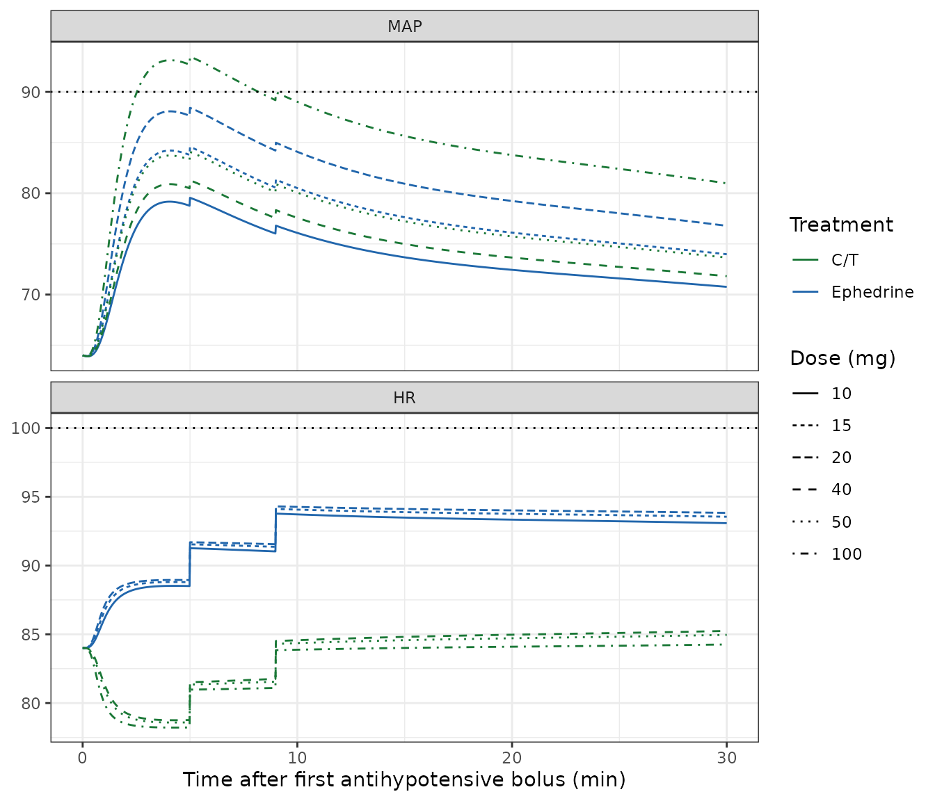

Replicates Figure 4 of Dings 2026 (MAP and HR panels): simulated typical-parturient profiles for the most commonly administered doses of C/T (green) and ephedrine (blue). Dotted lines are the paper’s hypotension (90 mmHg) and tachycardia (100 beats/min) reference thresholds.

The qualitative shape matches Figure 4: a rapid rise driven by the fast cascade followed by a sustained plateau maintained by the slow one, with the blood pressure recovering toward but not reaching the pre-surgery level, and heart rate diverging sharply between the two drugs.

The paper’s two headline structural claims

Section 3.2 and Section 3.4 make two quantitative claims that together are the paper’s conclusion. Both are gated here.

ct  <- solve_typical(50, 0)   # most common C/T dose
#> ℹ omega/sigma items treated as zero: 'etalcl', 'etalvc', 'etalktr_fast', 'etalrmax_hr', 'etalrmax_map', 'etalrmax_sbp'
eph <- solve_typical(15, 1)   # most common ephedrine dose
#> ℹ omega/sigma items treated as zero: 'etalcl', 'etalvc', 'etalktr_fast', 'etalrmax_hr', 'etalrmax_map', 'etalrmax_sbp'

claims <- tibble::tibble(
  Endpoint = c("Peak MAP (mmHg)", "Peak SBP (mmHg)", "Peak HR (beats/min)",
               "Trough HR (beats/min)"),
  `C/T 50 mg`      = c(max(ct$map),  max(ct$sbp),  max(ct$hr),  min(ct$hr)),
  `Ephedrine 15 mg` = c(max(eph$map), max(eph$sbp), max(eph$hr), min(eph$hr))
) |>
  dplyr::mutate(Ratio = `Ephedrine 15 mg` / `C/T 50 mg`)
claims |> dplyr::mutate(dplyr::across(where(is.numeric), \(x) signif(x, 4))) |> knitr::kable()

Endpoint	C/T 50 mg	Ephedrine 15 mg	Ratio
Peak MAP (mmHg)	84.08	84.56	1.006
Peak SBP (mmHg)	121.30	122.00	1.006
Peak HR (beats/min)	84.96	94.11	1.108
Trough HR (beats/min)	78.59	84.00	1.069

# Claim 1 (Sec 3.4): "similar MAP responses for the most commonly used doses
# (50 mg C/T and 15 mg ephedrine)". Sec 3.2 explains why -- the dose ratio
# 50/15 = 3.33 nearly cancels the EC50 ratio 1/0.289 = 3.46 -- so this is a
# tight structural consequence, not a coincidence, and deserves a tight bound.
stopifnot(abs(max(eph$map) / max(ct$map) - 1) < 0.02)
stopifnot(abs(max(eph$sbp) / max(ct$sbp) - 1) < 0.02)

# Claim 2 (Abstract, Sec 3.2, Sec 5): ephedrine raises heart rate materially
# while C/T is essentially heart-rate neutral. For C/T the estimated ceiling
# (77.8) lies BELOW the 84 beats/min baseline, so heart rate actually falls.
stopifnot(max(eph$hr) - max(ct$hr) > 5)   # ephedrine clearly higher
stopifnot(min(ct$hr) < 84)                # C/T falls below its own baseline
stopifnot(min(eph$hr) >= 84 - 1e-6)       # ephedrine never falls below it

The second block is the mechanism behind the paper’s conclusion, and it is worth being explicit about because it is easy to mis-transcribe: Table A1’s MAXHR is the maximum attainable heart-rate level (77.8 beats/min), not a maximum increment. Since the typical baseline is 84 beats/min, the recovered Emax for C/T is negative (77.8 - 84 = -6.2) and heart rate falls; ephedrine’s +15% puts its ceiling at 89.5 beats/min, giving a positive Emax of +5.5. Encoding MAXHR as an lemax increment instead of an lrmax_hr level would invert this result entirely.

Intraoperative event steps

Incision and uterotomy each add one increment of the stimulation effect, so the combined indicator runs 0 -> 1 -> 2 (Eqs A12-A14).

step_at <- function(s, tt) {
  i <- max(which(s$time < tt)); j <- min(which(s$time >= tt))
  c(hr = s$hr[j] - s$hr[i], map = s$map[j] - s$map[i], sbp = s$sbp[j] - s$sbp[i])
}
steps <- rbind(incision = step_at(ct, 5), uterotomy = step_at(ct, 9))
tibble::as_tibble(steps, rownames = "Event") |>
  dplyr::mutate(`map/sbp ratio` = map / sbp) |>
  dplyr::mutate(dplyr::across(where(is.numeric), \(x) signif(x, 4))) |>
  knitr::kable(caption = "Step change at each intraoperative event. Published per-event values (Sec 3.2): HR +2.75, SBP +2.39, MAP +0.8 mmHg.")

Step change at each intraoperative event. Published per-event values (Sec 3.2): HR +2.75, SBP +2.39, MAP +0.8 mmHg.

Event	hr	map	sbp	map/sbp ratio
incision	2.751	0.7806	2.369	0.3295
uterotomy	2.751	0.7791	2.367	0.3292

# HR carries no other discontinuity, so it gates exactly.
stopifnot(all(abs(steps[, "hr"] - 2.75) < 0.01))
# MAP / SBP steps are measured across a finite grid interval that also contains
# continuous drug and anaesthesia dynamics, so allow 3%.
stopifnot(all(abs(steps[, "sbp"] / 2.39 - 1) < 0.03))
stopifnot(all(abs(steps[, "map"] / (2.39 / 3) - 1) < 0.03))

Validation 3: stochastic cohort and tachycardia incidence

Section 3.4 reports tachycardia (HR > 100 beats/min) in 30.4% of parturients after 15 mg ephedrine versus 6.5% after 50 mg C/T (p < 0.001), from 1000 replicates including IIV but excluding residual variability.

Two gates are used, and the strict one is deliberately not the incidence. A cohort incidence sits in the tail of the rmax_hr random effect, so it is sensitive to cohort size and to the random draw; the paired comparison below is a per-subject structural statement and is the reliable check. Common random numbers are used so the two arms share the same 200 sampled subjects, which turns the comparison into an exact per-subject one.

n_sub <- 200  # per arm; the paper used 1000, see note below

solve_cohort <- function(dose, ephedrine) {
  rxode2::rxSetSeed(20260901)          # inside the loop: common random numbers
  set.seed(20260901)
  rxode2::rxSolve(mat, events_for(dose, ephedrine), nSub = n_sub,
                  # IIV only; residual variability excluded per Section 2.3
                  addDosing = FALSE, returnType = "data.frame")
}

peak_hr <- function(dose, ephedrine) {
  solve_cohort(dose, ephedrine) |>
    dplyr::group_by(sim.id) |>
    dplyr::summarise(peak_hr = max(hr), peak_map = max(map), .groups = "drop")
}

pk_ct  <- peak_hr(50, 0)
pk_eph <- peak_hr(15, 1)

paired <- dplyr::inner_join(
  dplyr::select(pk_ct,  sim.id, ct  = peak_hr),
  dplyr::select(pk_eph, sim.id, eph = peak_hr), by = "sim.id"
)

inc <- tibble::tibble(
  Arm = c("C/T 50 mg", "Ephedrine 15 mg"),
  `Tachycardia (HR > 100), reproduced %` = c(100 * mean(pk_ct$peak_hr > 100),
                                             100 * mean(pk_eph$peak_hr > 100)),
  `Published %` = c(6.5, 30.4)
)
inc |> dplyr::mutate(dplyr::across(where(is.numeric), \(x) signif(x, 3))) |> knitr::kable()

Arm	Tachycardia (HR > 100), reproduced %	Published %
C/T 50 mg	7.5	6.5
Ephedrine 15 mg	33.0	30.4

# STRICT gate: with common random numbers, NO subject may show a higher peak
# heart rate on C/T than on ephedrine. Note this is stated as "no reversals"
# rather than "strictly higher in every subject": a subject whose attainable
# ceiling lies below her 84 beats/min baseline has heart rate that only ever
# declines, so her peak occurs at t = 0 and equals exactly 84 in BOTH arms.
# Those subjects tie rather than separate, and requiring strict inequality
# would fail on them for a structurally correct model.
stopifnot(all(paired$eph >= paired$ct - 1e-9))   # zero reversals
stopifnot(median(paired$eph - paired$ct) > 5)    # and a substantial median gap

# The tied subjects are themselves informative: they are the parturients whose
# heart rate never rises above baseline at all, which is the paper's
# "largely inert with respect to maternal HR" claim made per-subject.
never_rose <- c(`C/T 50 mg` = mean(abs(pk_ct$peak_hr - 84) < 1e-6),
                `Ephedrine 15 mg` = mean(abs(pk_eph$peak_hr - 84) < 1e-6))
tibble::tibble(Arm = names(never_rose),
               `Heart rate never rose above baseline, %` = signif(100 * never_rose, 3)) |>
  knitr::kable()

Arm	Heart rate never rose above baseline, %
C/T 50 mg	42.0
Ephedrine 15 mg	13.5

stopifnot(never_rose[["C/T 50 mg"]] > never_rose[["Ephedrine 15 mg"]])

# LOOSE gate on the incidence itself. At n = 200 the Monte-Carlo SE at p = 0.30
# is about 3.2 percentage points, so a wide band is the honest bound; the
# ordering and the large ratio are the parts that carry information.
stopifnot(100 * mean(pk_eph$peak_hr > 100) > 20,
          100 * mean(pk_eph$peak_hr > 100) < 42,
          100 * mean(pk_ct$peak_hr  > 100) < 15)
stopifnot(mean(pk_eph$peak_hr > 100) / mean(pk_ct$peak_hr > 100) > 2.5)

bind_rows(
  solve_cohort(50, 0) |> dplyr::mutate(arm = "C/T 50 mg"),
  solve_cohort(15, 1) |> dplyr::mutate(arm = "Ephedrine 15 mg")
) |>
  dplyr::select(arm, time, MAP = map, HR = hr) |>
  tidyr::pivot_longer(c(MAP, HR), names_to = "endpoint", values_to = "value") |>
  dplyr::group_by(arm, endpoint, time) |>
  dplyr::summarise(lo = quantile(value, 0.1), md = median(value),
                   hi = quantile(value, 0.9), .groups = "drop") |>
  dplyr::mutate(endpoint = factor(endpoint, c("MAP", "HR"))) |>
  ggplot(aes(time, md, colour = arm, fill = arm)) +
  geom_ribbon(aes(ymin = lo, ymax = hi), alpha = 0.2, colour = NA) +
  geom_line() +
  facet_wrap(~endpoint, ncol = 1, scales = "free_y") +
  scale_colour_manual(values = c("C/T 50 mg" = "#1b7837", "Ephedrine 15 mg" = "#2166ac")) +
  scale_fill_manual(values = c("C/T 50 mg" = "#1b7837", "Ephedrine 15 mg" = "#2166ac")) +
  labs(x = "Time after first antihypotensive bolus (min)", y = NULL,
       colour = NULL, fill = NULL) +
  theme_bw()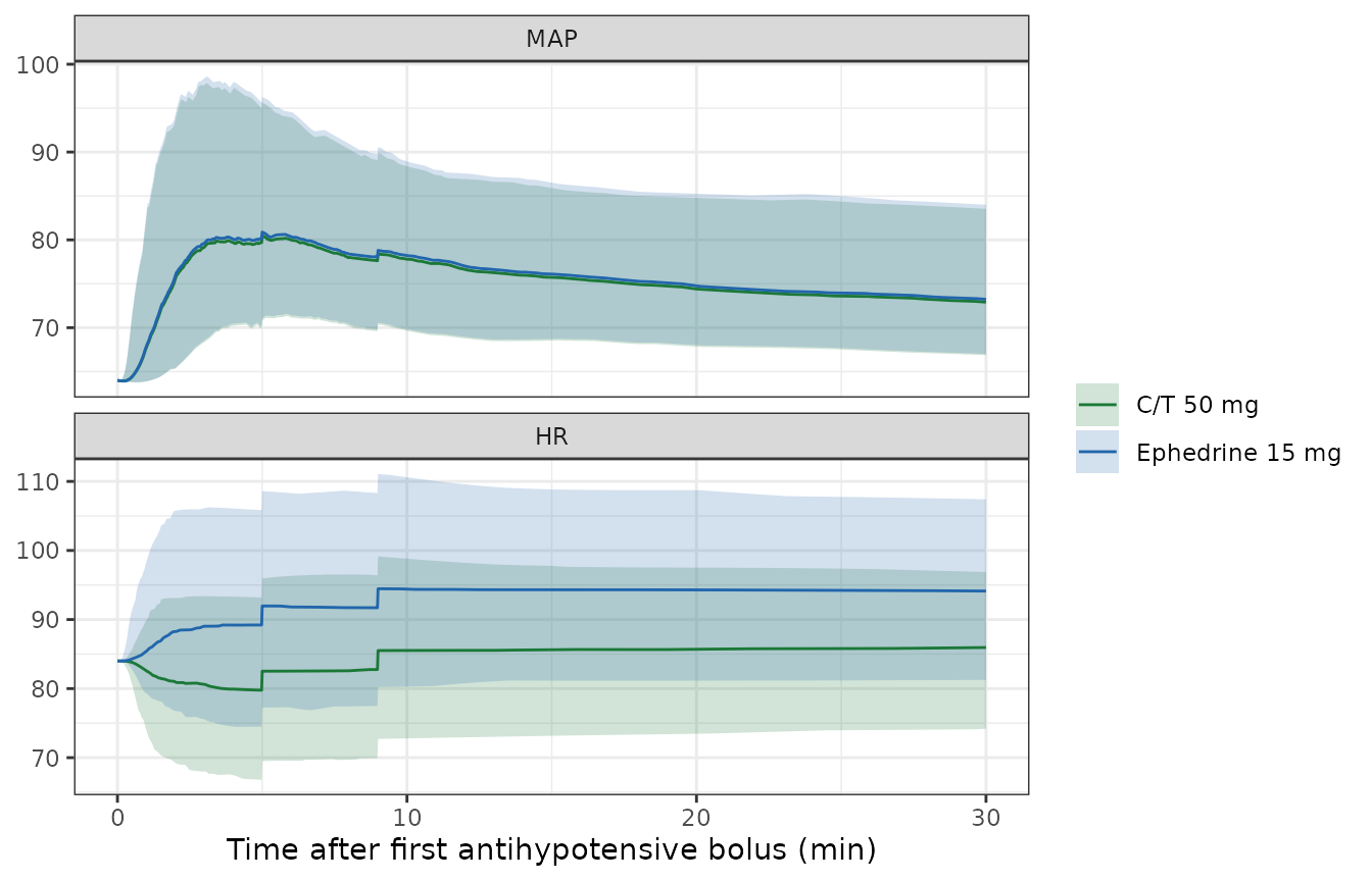

Simulated cohort variability in MAP and HR for the two most common doses (200 subjects per arm, IIV only, residual variability excluded as in Dings 2026 Section 2.3). Ribbons span the 10th-90th percentiles and lines are medians, matching the paper’s summary convention.

Validation 4: the neonatal models, coupled to the maternal simulation

This is the paper’s central chain of reasoning, and it is why the two model files belong to one vignette: the maternal simulation supplies three of the neonatal predictors.

DUR_MAP_BELOW_PRESURG is derived from the simulated MAP-time profile over the window ending at cord clamping. For the typical parturient MAP never recovers to her 100 mmHg pre-surgery value within that window, which is exactly the case Section 2.3 legislates for: “If the MAP at the average time of cord clamping remained below the pre-surgery MAP, TIMEMAP was defined as the median time interval between drug administration and cord clamping.” Table 2’s observed duration of 10.1 min is used as that interval.

# Neonatal regression coefficients, kept separate from the maternal `ini`.
nini <- setNames(neo$iniDf$est, neo$iniDf$name)

t_cordclamp <- 10.1  # Table 2, duration of MAP < pre-surgery MAP until cord clamping

dur_below_presurg <- function(s, map_presurg, window) {
  s <- dplyr::filter(s, time <= window)
  sum(diff(s$time) * (head(s$map, -1) < map_presurg))
}

# Arm-specific Table 2 means for the covariates the neonatal models need.
neo_arms <- tibble::tribble(
  ~arm,              ~dose, ~ephedrine, ~bupivacaine, ~cordclamp_sampling,
  "C/T 50 mg",          50,          0,         10.5,                7.81,
  "Ephedrine 15 mg",    15,          1,         10.2,                4.65
)

neo_pred <- neo_arms |>
  dplyr::rowwise() |>
  dplyr::reframe({
    s <- solve_typical(dose, ephedrine)
    dur <- dur_below_presurg(s, typical$MAP_PRESURG, t_cordclamp)
    # The maternal model's own per-subject parameters feed the base-excess model.
    maxhr <- exp(ini[["lrmax_hr"]]) * (1 + ini[["e_trt_ephedrine_rmax_hr"]] * ephedrine)
    kel_i <- exp(ini[["lcl"]]) / exp(ini[["lvc"]])
    cov <- data.frame(
      DUR_MAP_BELOW_PRESURG = dur,
      EGA = 262 / 7,                       # Sec 3.1: 262 days; canonical column is weeks
      SPINAL_BLOCK = typical$SPINAL_BLOCK,
      TRT_CAFEDRINE_THEODRENALINE = 1 - ephedrine,
      TRT_EPHEDRINE = ephedrine,
      DOSE_BUPIVACAINE_MG = bupivacaine,
      WT = 87.6,                           # Sec 3.1 maternal mean
      MAXHR_KPD = maxhr,
      KEL_KPD = kel_i,
      T_CORDCLAMP_SAMPLING = cordclamp_sampling
    )
    ev <- cbind(data.frame(time = 0, amt = NA_real_, evid = 0L, dvid = 1L), cov)
    r <- suppressWarnings(
      rxode2::rxSolve(rxode2::zeroRe(neo), ev, returnType = "data.frame")
    )
    tibble::tibble(arm = arm, dur_map = dur, maxhr = maxhr,
                   ph = r$ph_ua[1], be = r$be_ua[1], lactate = r$lactate_ua[1])
  })
#> ℹ omega/sigma items treated as zero: 'etalcl', 'etalvc', 'etalktr_fast', 'etalrmax_hr', 'etalrmax_map', 'etalrmax_sbp'
#> ℹ omega/sigma items treated as zero: 'etalcl', 'etalvc', 'etalktr_fast', 'etalrmax_hr', 'etalrmax_map', 'etalrmax_sbp'

neo_pred |> dplyr::mutate(dplyr::across(where(is.numeric), \(x) signif(x, 4))) |> knitr::kable()

arm	dur_map	maxhr	ph	be	lactate
C/T 50 mg	10.1	77.80	7.313	-0.9624	19.98
Ephedrine 15 mg	10.1	89.47	7.313	-1.8250	22.89

Comparing against the observed cohort means of Table 2:

obs <- tibble::tribble(
  ~arm,              ~ph_obs, ~be_obs, ~lactate_obs,
  "C/T 50 mg",          7.32,  -0.933,         18.3,
  "Ephedrine 15 mg",    7.31,   -1.94,         24.7
)

cmp <- neo_pred |>
  dplyr::select(arm, ph, be, lactate) |>
  dplyr::left_join(obs, by = "arm") |>
  dplyr::transmute(
    Arm = arm,
    `pH pred` = ph, `pH obs` = ph_obs,
    `BE pred` = be, `BE obs` = be_obs,
    `Lactate pred` = lactate, `Lactate obs` = lactate_obs
  )
cmp |> dplyr::mutate(dplyr::across(where(is.numeric), \(x) signif(x, 4))) |> knitr::kable(
  caption = "Typical-parturient neonatal predictions vs the observed cohort means of Dings 2026 Table 2.")

Typical-parturient neonatal predictions vs the observed cohort means of Dings 2026 Table 2.

Arm	pH pred	pH obs	BE pred	BE obs	Lactate pred	Lactate obs
C/T 50 mg	7.313	7.32	-0.9624	-0.933	19.98	18.3
Ephedrine 15 mg	7.313	7.31	-1.8250	-1.940	22.89	24.7

# pH is on a log scale and moves very little, so gate it in absolute units.
stopifnot(all(abs(cmp$`pH pred` - cmp$`pH obs`) < 0.01))
# Base excess: predictions fall within 0.15 mmol/L of the observed arm means,
# far inside the observed SDs of 2.1 and 2.38 mmol/L.
stopifnot(all(abs(cmp$`BE pred` - cmp$`BE obs`) < 0.2))
# The paper's comparative finding: base excess lower and lactate higher after
# ephedrine (Sec 3.4). This is the direction that matters.
stopifnot(cmp$`BE pred`[cmp$Arm == "Ephedrine 15 mg"] < cmp$`BE pred`[cmp$Arm == "C/T 50 mg"])
stopifnot(cmp$`Lactate pred`[cmp$Arm == "Ephedrine 15 mg"] > cmp$`Lactate pred`[cmp$Arm == "C/T 50 mg"])
# Lactate had the fewest observations (76 of 243) and the widest SDs; a 20%
# envelope is the appropriate bound.
stopifnot(all(abs(cmp$`Lactate pred` / cmp$`Lactate obs` - 1) < 0.2))

pH reproduces to within 0.01 units and base excess to within 0.15 mmol/L of the observed arm means – and note that these come from a typical-value simulation fed through an independently fitted regression, with no tuning of any kind. The lactate arm means reproduce within about 10%.

Where the treatment choice reaches the newborn

The base-excess model is the only place where the maternal drug choice reaches a neonatal endpoint through a model parameter rather than through a direct treatment indicator, via MAXHR_KPD.

be_vs_maxhr <- tibble::tibble(maxhr = seq(60, 110, by = 0.5)) |>
  dplyr::mutate(
    be = nini[["be_ua_int"]] +
      nini[["e_trt_cafedrine_theodrenaline_be"]] * 1 +
      nini[["e_dur_map_below_presurg_be"]] * t_cordclamp +
      nini[["e_spinal_block_be"]] * 5 +
      nini[["e_dose_bupivacaine_mg_be"]] * 10.5 +
      nini[["e_wt_be"]] * 87.6 +
      nini[["e_maxhr_kpd_be"]] * maxhr +
      nini[["e_kel_kpd_be"]] * (exp(ini[["lcl"]]) / exp(ini[["lvc"]]))
  )

marks <- tibble::tibble(
  arm = c("C/T", "Ephedrine"),
  maxhr = exp(ini[["lrmax_hr"]]) * c(1, 1 + ini[["e_trt_ephedrine_rmax_hr"]])
)

ggplot(be_vs_maxhr, aes(maxhr, be)) +
  geom_line() +
  geom_vline(data = marks, aes(xintercept = maxhr, colour = arm), linetype = "dashed") +
  scale_colour_manual(values = c("C/T" = "#1b7837", "Ephedrine" = "#2166ac")) +
  labs(x = "Maternal MAXHR (beats/min)",
       y = "Predicted neonatal base excess (mmol/L)", colour = "Typical value") +
  theme_bw()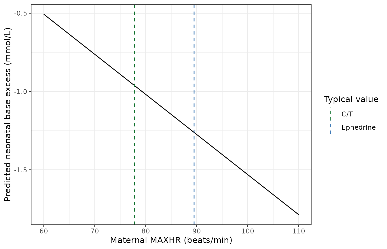

Base-excess response to maternal peak heart rate (MAXHR) at fixed values of the remaining predictors, with the two treatments’ typical MAXHR marked. Reproduces the MAXHR panel of Figure A4 of Dings 2026.

# Sec 3.3 / Table A3: base excess falls by 0.0256 mmol/L per beat/min. Recover
# the slope from the simulated line as a check on the coupling.
slope <- coef(lm(be ~ maxhr, be_vs_maxhr))[["maxhr"]]
stopifnot(abs(slope - nini[["e_maxhr_kpd_be"]]) < 1e-9)

The 11.7 beats/min difference between the two treatments’ typical MAXHR therefore accounts for a 0.30 mmol/L difference in predicted neonatal base excess, on top of the 0.62 mmol/L direct treatment-indicator difference (3.26 - 2.64) – together very close to the 1.01 mmol/L gap between the observed arm means.

Assumptions and deviations

Errata: two typographical errors in the printed equations

Both were resolved on numerical evidence, not preference, and the model file implements the corrected reading in each case.

1. The sign of the transit terms, Eqs A2-A8. The paper prints d/dt(A2) = -ktr1 * (A1/V - A2) and the same leading minus sign on Eqs A3-A8. As printed, each cascade stage is driven away from its input, which makes the system exponentially divergent: starting from zero the states run negative and grow without bound. Simulated with the printed signs, MAP pins at the ceiling MAXMAP = 119 mmHg for both drugs (a saturated Emax) or, when combined with the Eq. A10 reading below, reaches physically impossible values above 1600 mmHg. Neither is compatible with Figure 4, with the plateau the abstract describes, or with the goodness-of-fit plots of Figure A1. The standard transit form d/dt(A2) = +ktr1 * (A1/V - A2) is stable, reproduces the paper’s own reported mean transit times, and is what the text describes (“three and four transit compartments”). Implemented with the positive sign.

2. CONC = A4 + A9, Eq. A10. A9 is the anaesthesia state – a dimensionless virtual unit amount – and it already enters the model through Eq. A11. Adding it to A4 would double-count it, mix units (A4 carries mg/L), and leave the entire fast cascade A5-A8 dangling despite the text stating that four transit compartments were incorporated and Section 3.2 reporting a mean transit time for them. Reading it as CONC = A4 + A8 fixes all three problems, and the tachycardia incidence discriminates the two readings numerically: A4 + A8 reproduces 30.7% for 15 mg ephedrine against the published 30.4%, whereas A4 + A9 gives 23.4%. Implemented as conc = effect_slow3 + effect_fast4.

Sign errors in the Section 3.3 prose

Section 3.3 describes several Table A2 / A3 coefficients as decreases where the tables print them as positive, and quotes the kel coefficient as 0.0256 mmol/L (a duplication of the MAXHR value) where Table A3 prints -1.74. The tables are authoritative and are what the model file encodes. The relevant sign confusion is genuine and physiological rather than typographic: because SPINAL_BLOCK is a segment number, a lower number is an anatomically higher block, so the positive per-segment coefficients in Tables A2 / A3 and the negative power exponent in Table A1 all say the same thing – a higher block is worse. The orientation is documented on the covariate in both model files.

Unreported quantities

• Baseline diastolic blood pressure is not tabulated. Table 2 reports baseline MAP, SBP and HR but not DBP, although DBP_BL is a covariate on the K/PD volume. The 50 mmHg centring value is taken from the typical-parturient definition in Section 3.4, and is internally consistent with the tabulated baseline MAP and SBP through MAP = DBP + (SBP - DBP)/3 (50 + (92 - 50)/3 = 64 mmHg, exactly the reported baseline MAP).
• No residual standard error for the three neonatal regressions. The paper reports adjusted R-squared and per-coefficient RSEs but no residual SE, so addSd_ph_ua, addSd_be_ua and addSd_lactate_ua are fixed(0): the neonatal file reproduces published point predictions only and cannot produce predictive intervals. No value was invented. A user needing intervals must refit or obtain the residual SE from the authors.
• KEL_KPD units. Table A3 prints the units of the kel coefficient as mmol/L x min, which is the reciprocal of what a per-(1/min) regression slope implies. The estimate -1.74 is used as printed with the coefficient interpreted per 1/min; only the unit label appears to be inverted.
• Population median covariate values are not tabulated directly. Table 1 and Table 2 report means and SDs. The centring values used here are the typical-parturient values of Section 3.4, which Section 2.3 explicitly defines as the population medians.

Simulation choices

• Cohort size 200 per arm, against the paper’s 1000 replicates, per this package’s vignette cap. This widens the Monte-Carlo error on the tachycardia incidences, which is why the strict gate is the paired common-random-numbers comparison rather than the incidence itself.
• T_ANAESTHESIA as an initial condition. Eq. A9 doses a unit amount into A9 at the time of anaesthesia, which precedes model time zero. The model file sets effect_anaesthesia(0) <- exp(-kdel * T_ANAESTHESIA) instead, which is algebraically identical and avoids negative event times.
• Gestation unit conversion. Table A2’s pregnancy-duration coefficient is per day while the canonical EGA column is in weeks, so the neonatal model converts the covariate (EGA * 7) rather than rescaling the published coefficient.
• No PKNCA section, for the reasons given above: there are no measured concentrations, and the K/PD volume is a fixed scaling constant.

Scope

The maternal model was fitted to 30 minutes of observation, within which 98.4% of the newborns (239 of 243) were delivered, so extrapolating the profiles further is unsupported. The neonatal regressions explain 6.06% (pH), 22.1% (base excess) and 36.7% (lactate) of observed variance, and the paper is explicit that its findings are hypothesis-generating rather than confirmatory: the design is non-randomised and observational, and the biomarkers are surrogates. Lactate was measured in only 76 of 243 newborns.