Piperacillin + tazobactam in healthy adults (Lee 2025)
Source:vignettes/articles/Lee_2025_piperacillin_tazobactam.Rmd
Lee_2025_piperacillin_tazobactam.RmdModel and source
Lee 2025 fitted piperacillin and tazobactam separately, in two independent NONMEM runs with their own structural, covariate, IIV and residual-error structures (Tables 2 and 3 of the paper). Following the library’s replicate-the-author’s-structure policy, the paper therefore contributes two model files, which this single vignette validates side by side.
pip <- rxode2::rxode(readModelDb("Lee_2025_piperacillin"))
#> ℹ parameter labels from comments will be replaced by 'label()'
taz <- rxode2::rxode(readModelDb("Lee_2025_tazobactam"))
#> ℹ parameter labels from comments will be replaced by 'label()'- Citation: Lee YJ, Kang G, Zang DY, Lee DH. Population pharmacokinetic modeling of piperacillin/tazobactam in healthy adults and exploration of optimal dosing strategies. Pharmaceuticals (Basel). 2025;18(8):1124. doi:10.3390/ph18081124. Structural model, covariate equations and all parameter estimates: Table 2. Covariate-selection path: Table A1.
- Piperacillin model: Two-compartment population PK model for piperacillin in 12 healthy Korean adults given a single 4 g / 0.5 g piperacillin-tazobactam IV infusion over 30 min (Lee 2025); zero-order IV input into the central compartment, first-order elimination, a power effect of BSA-adjusted CKD-EPI creatinine eGFR on CL, a power effect of lean body mass on Q (with the typical Q fixed), and an exponential effect of body weight on the peripheral volume V2.
- Tazobactam model: Two-compartment population PK model for tazobactam in 12 healthy Korean adults given a single 4 g / 0.5 g piperacillin-tazobactam IV infusion over 30 min (Lee 2025); zero-order IV input into the central compartment, first-order elimination, a power effect of BSA-adjusted CKD-EPI creatinine eGFR on CL, a fixed typical intercompartmental clearance Q, and an exponential effect of body weight on the peripheral volume V2.
- Article: https://doi.org/10.3390/ph18081124
The paper’s own dosing-exploration tool is available at https://dhlee.shinyapps.io/pthv/.
Population
Twelve healthy Korean adults (8 male, 4 female) received a single intravenous dose of 4 g piperacillin / 0.5 g tazobactam in 100 mL saline over 30 minutes at the Clinical Trial Center of Hallym University Sacred Heart Hospital in January 2023 (IRB 2022-08-006; trial registration KCT0009855). Plasma was sampled before the dose and at 0.5, 0.75, 1, 2, 3 and 6 hours after the start of the infusion and assayed by LC-MS/MS, giving 84 plasma samples in total (Lee 2025 Section 4.2, Section 2.2).
Baseline characteristics (Lee 2025 Table 1, reported as median with range) were age 36.0 years (26.0-50.0), weight 61.7 kg (45.8-88.5), height 168 cm (158-182), lean body mass 50.1 kg (36.6-65.9) and body surface area 1.71 m^2 (1.44-2.07). Renal function was normal throughout: Cockcroft-Gault CrCl 105 mL/min (76.2-146) and BSA-adjusted CKD-EPI creatinine eGFR 108 mL/min (86.2-136). All baseline laboratory values were within normal clinical ranges and no adverse drug reactions occurred.
The same information is available programmatically from either
model’s population metadata:
str(pip$population)
#> List of 17
#>  $ species       : chr "human"
#>  $ n_subjects    : num 12
#>  $ n_studies     : num 1
#>  $ age_range     : chr "26-50 years (inclusion criteria 19-55 years)"
#>  $ age_median    : chr "36.0 years"
#>  $ weight_range  : chr "45.8-88.5 kg"
#>  $ weight_median : chr "61.7 kg"
#>  $ sex_female_pct: num 33.3
#>  $ race_ethnicity: chr "Korean (all participants)"
#>  $ disease_state : chr "Healthy adults with no congenital or chronic health conditions; all baseline laboratory values within normal clinical ranges"
#>  $ dose_range    : chr "Single 4 g piperacillin / 0.5 g tazobactam intravenous dose in 100 mL saline, infused over 30 min"
#>  $ regions       : chr "Republic of Korea (Clinical Trial Center, Hallym University Sacred Heart Hospital, Anyang)"
#>  $ renal_function: chr "Normal; CrCl (Cockcroft-Gault) 105 mL/min (76.2-146), BSA-adjusted CKD-EPI creatinine eGFR 108 mL/min (86.2-136)"
#>  $ height_range  : chr "158-182 cm (median 168)"
#>  $ lbm_range     : chr "36.6-65.9 kg (median 50.1)"
#>  $ bsa_range     : chr "1.44-2.07 m^2 (median 1.71)"
#>  $ notes         : chr "12 healthy Korean adults (8 male, 4 female) studied in January 2023; IRB 2022-08-006, trial registration KCT000"| __truncated__
Source trace
Every ini() entry in the two model files carries an
in-file comment pointing at its source location. The tables below
collect them for review.
Piperacillin (Lee 2025 Table 2)
| Equation / parameter | Value | Source location |
|---|---|---|
CL = theta1 * (CE / 108.25)^theta2 |
structural | Table 2, “Structural model” row |
lcl (theta1) |
11.2 L/h | Table 2 (RSE 3.40%; bootstrap 11.2, 95% CI 10.5-12.1) |
e_crcl_cl (theta2) |
1.16 | Table 2 (RSE 13.1%; bootstrap 1.15, 95% CI 0.811-1.59) |
crcl_ref |
108.25 mL/min | Table 2 equation; cohort median in Table 1 (108) |
V1 = theta3; lvc
|
6.24 L | Table 2 (RSE 8.99%; bootstrap 6.19, 95% CI 5.27-7.57) |
Q = theta4 * (LBM / 50.08)^theta5 |
structural | Table 2 |
lq (theta4) |
4.32 L/h, FIXED | Table 2, footnote a (“fixed”; no RSE, no bootstrap CI) |
e_lbm_q (theta5) |
2.50 | Table 2 (RSE 13.9%; bootstrap 2.45, 95% CI 1.39-3.56) |
lbm_ref |
50.08 kg | Table 2 equation; cohort median in Table 1 (50.1) |
V2 = theta6 * exp(theta7 * (WT - 61.7)) |
structural | Table 2 |
lvp (theta6) |
2.59 L | Table 2 (RSE 3.11%; bootstrap 2.59, 95% CI 2.28-2.74) |
e_wt_vp (theta7) |
0.0288 per kg | Table 2 (RSE 8.38%; bootstrap 0.0284, 95% CI 0.0208-0.0371) |
wt_ref |
61.7 kg | Table 2 equation; cohort median in Table 1 |
etalcl |
7.17% -> var 0.00512772 | Table 2 IIV CL (RSE 30.3%, shrinkage 18.7%) |
etalvc |
18.4% -> var 0.03329550 | Table 2 IIV V1 (RSE 28.7%, shrinkage 19.1%) |
propSd |
0.134 | Table 2 proportional error 13.4% (RSE 12.2%, shrinkage 9.48%) |
| Covariate-selection path | n/a | Table A1 (forward selection + backward elimination) |
Tazobactam (Lee 2025 Table 3)
| Equation / parameter | Value | Source location |
|---|---|---|
CL = theta1 * (CE / 108.25)^theta2 |
structural | Table 3, “Structural model” row |
lcl (theta1) |
12.4 L/h | Table 3 (RSE 3.26%; bootstrap 12.3, 95% CI 11.6-13.3) |
e_crcl_cl (theta2) |
0.857 | Table 3 (RSE 13.1%; bootstrap 0.858, 95% CI 0.602-1.21) |
crcl_ref |
108.25 mL/min | Table 3 equation; cohort median in Table 1 (108) |
V1 = theta3; lvc
|
9.03 L | Table 3 (RSE 6.40%; bootstrap 9.02, 95% CI 8.05-10.4) |
Q = theta4; lq
|
4.39 L/h, FIXED | Table 3, footnote a (“fixed”; no RSE, no bootstrap CI) |
V2 = theta5 * exp(theta6 * (WT - 61.7)) |
structural | Table 3 |
lvp (theta5) |
3.21 L | Table 3 (RSE 5.48%; bootstrap 3.23, 95% CI 2.68-3.48) |
e_wt_vp (theta6) |
0.0145 per kg | Table 3 (RSE 16.9%; bootstrap 0.0142, 95% CI 0.0106-0.0238) |
wt_ref |
61.7 kg | Table 3 equation; cohort median in Table 1 |
etalcl |
6.95% -> var 0.00481862 | Table 3 IIV CL (RSE 29.0%, shrinkage 7.37%) |
(no etalvc) |
dropped | Section 2.2: IIV on V1 excluded, RSE > 70% |
propSd |
0.135 | Table 3 proportional error 13.5% (RSE 9.57%, shrinkage 6.06%) |
| Covariate-selection path | n/a | Table A2 (forward selection + backward elimination) |
Two scale decisions in the tables above deserve a note.
-
The IIV column is on the SD scale, not the variance
scale. With
n = 12subjects, the %RSE of a variance estimate cannot fall belowsqrt(2/12) = 40.8%; the reported IIV %RSEs are 30.3%, 28.7% and 29.0%, all below that floor, so the column cannot be a variance. It is converted here withomega^2 = log(1 + CV^2). -
theta4(Q) is fixed in both models. Table 2 and Table 3 mark it with footnotea(“fixed”) and report neither an RSE nor a bootstrap interval for it, unlike every other estimated parameter. It is wrapped infixed()in both model files.
Virtual cohort
The original concentration data are not publicly available (Lee 2025 Data Availability Statement), so the checks below use a virtual cohort whose covariate distributions approximate Table 1.
set.seed(20250727)

n_arm <- 200

# Log-normal draws pinned to the Table 1 sex-specific medians, with a spread
# chosen so ~95% of draws fall inside the reported ranges.
rln <- function(n, median, sd_log) exp(rnorm(n, log(median), sd_log))

make_subjects <- function(n_f, n_m, id_offset = 0L) {
  female <- tibble(
    SEXF = 1L,
    WT   = rln(n_f, 56.1, 0.075),
    CRCL = rln(n_f, 108,  0.075)
  ) |>
    mutate(LBM = WT * (42.6 / 56.1))
  male <- tibble(
    SEXF = 0L,
    WT   = rln(n_m, 69.1, 0.105),
    CRCL = rln(n_m, 110,  0.090)
  ) |>
    mutate(LBM = WT * (55.2 / 69.1))
  bind_rows(female, male) |>
    mutate(id = id_offset + row_number()) |>
    select(id, SEXF, WT, LBM, CRCL)
}

# One arm: 1/3 female, 2/3 male, matching the 4-female / 8-male study cohort.
subjects <- make_subjects(n_f = round(n_arm / 3), n_m = n_arm - round(n_arm / 3))

subjects |>
  summarise(
    across(c(WT, LBM, CRCL),
           list(median = ~median(.x), min = ~min(.x), max = ~max(.x)))
  ) |>
  pivot_longer(everything(), names_to = c("covariate", "stat"),
               names_sep = "_(?=median|min|max)") |>
  pivot_wider(names_from = stat, values_from = value) |>
  rename("Covariate" = covariate, "Median" = median,
         "Minimum" = min, "Maximum" = max) |>
  knitr::kable(
    digits = 1,
    caption = paste(
      "Simulated cohort covariates. Lee 2025 Table 1 reports WT 61.7 (45.8-88.5) kg,",
      "LBM 50.1 (36.6-65.9) kg, BSA-adjusted CKD-EPI eGFR 108 (86.2-136) mL/min."
    )
)| Covariate | Median | Minimum | Maximum |
|---|---|---|---|
| WT | 63.1 | 43.7 | 98.6 |
| LBM | 50.1 | 33.2 | 78.8 |
| CRCL | 110.0 | 90.5 | 143.1 |
The event table reproduces the study design: a single 4 g
piperacillin / 0.5 g tazobactam intravenous dose infused over 30
minutes, observed on the central compartment.
dose_dur <- 0.5   # h, Lee 2025 Section 4.2
obs_grid <- sort(unique(c(seq(0, 8, by = 0.05), dose_dur)))

make_events <- function(subjects, amt, dur = dose_dur, times = obs_grid) {
  dosing <- subjects |>
    mutate(time = 0, amt = amt, evid = 1L, rate = amt / dur, cmt = "central")
  observations <- subjects |>
    tidyr::crossing(time = times) |>
    mutate(amt = NA_real_, evid = 0L, rate = 0, cmt = "central")
  bind_rows(dosing, observations) |>
    arrange(id, time, desc(evid))
}

ev_pip <- make_events(subjects, amt = 4000)   # mg piperacillin
ev_taz <- make_events(subjects, amt =  500)   # mg tazobactam

stopifnot(!anyDuplicated(unique(ev_pip[, c("id", "time", "evid")])))
stopifnot(!anyDuplicated(unique(ev_taz[, c("id", "time", "evid")])))
Simulation
sim_pip <- rxode2::rxSolve(
  readModelDb("Lee_2025_piperacillin"), events = ev_pip,
  keep = c("WT", "LBM", "CRCL", "SEXF")
) |>
  as.data.frame() |>
  mutate(analyte = "Piperacillin 4 g")
#> ℹ parameter labels from comments will be replaced by 'label()'

sim_taz <- rxode2::rxSolve(
  readModelDb("Lee_2025_tazobactam"), events = ev_taz,
  keep = c("WT", "LBM", "CRCL", "SEXF")
) |>
  as.data.frame() |>
  mutate(analyte = "Tazobactam 0.5 g")
#> ℹ parameter labels from comments will be replaced by 'label()'

# rxSolve drops `id` for a single-subject event table; guard against that here
# so the assertion below is never vacuous.
stopifnot(dplyr::n_distinct(sim_pip$id) == n_arm,
          dplyr::n_distinct(sim_taz$id) == n_arm)

sim_both <- bind_rows(sim_pip, sim_taz)
Replicate published figures
Figure 1 - concentration-time profiles
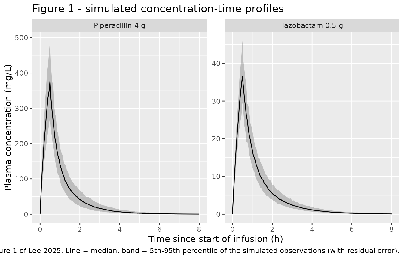
Cc is the individual prediction; the sim
column additionally carries the proportional residual error, so it is
the quantity comparable to the observed points plotted in Lee 2025
Figure 1.
# Replicates Figure 1 of Lee 2025: piperacillin (a) and tazobactam (b)
# concentration-time profiles in healthy adults after a single 4 g / 0.5 g
# intravenous dose infused over 30 min.
sim_both |>
  group_by(analyte, time) |>
  summarise(
    Q05 = quantile(sim, 0.05),
    Q50 = quantile(sim, 0.50),
    Q95 = quantile(sim, 0.95),
    .groups = "drop"
  ) |>
  ggplot(aes(time, Q50)) +
  geom_ribbon(aes(ymin = Q05, ymax = Q95), alpha = 0.25) +
  geom_line() +
  facet_wrap(~analyte, scales = "free_y") +
  scale_x_continuous(breaks = seq(0, 8, by = 2)) +
  labs(
    x = "Time since start of infusion (h)",
    y = "Plasma concentration (mg/L)",
    title = "Figure 1 - simulated concentration-time profiles",
    caption = paste(
      "Replicates Figure 1 of Lee 2025. Line = median, band = 5th-95th",
      "percentile of the simulated observations (with residual error)."
    )
  )
Covariate relationships (Tables 2 and 3 structural equations)
typ <- function(model_name) {
  ui <- rxode2::rxode(readModelDb(model_name))
  setNames(ui$theta, names(ui$theta))
}
th_pip <- typ("Lee_2025_piperacillin")
#> ℹ parameter labels from comments will be replaced by 'label()'
th_taz <- typ("Lee_2025_tazobactam")
#> ℹ parameter labels from comments will be replaced by 'label()'

cov_curves <- bind_rows(
  tibble(
    analyte = "Piperacillin", parameter = "CL (L/h)",
    x = seq(40, 180, length.out = 100)
  ) |>
    mutate(y = exp(th_pip[["lcl"]]) * (x / 108.25)^th_pip[["e_crcl_cl"]],
           xlab = "BSA-adjusted eGFR (mL/min)"),
  tibble(
    analyte = "Tazobactam", parameter = "CL (L/h)",
    x = seq(40, 180, length.out = 100)
  ) |>
    mutate(y = exp(th_taz[["lcl"]]) * (x / 108.25)^th_taz[["e_crcl_cl"]],
           xlab = "BSA-adjusted eGFR (mL/min)"),
  tibble(
    analyte = "Piperacillin", parameter = "V2 (L)",
    x = seq(45, 90, length.out = 100)
  ) |>
    mutate(y = exp(th_pip[["lvp"]] + th_pip[["e_wt_vp"]] * (x - 61.7)),
           xlab = "Body weight (kg)"),
  tibble(
    analyte = "Tazobactam", parameter = "V2 (L)",
    x = seq(45, 90, length.out = 100)
  ) |>
    mutate(y = exp(th_taz[["lvp"]] + th_taz[["e_wt_vp"]] * (x - 61.7)),
           xlab = "Body weight (kg)"),
  tibble(
    analyte = "Piperacillin", parameter = "Q (L/h)",
    x = seq(36, 66, length.out = 100)
  ) |>
    mutate(y = exp(th_pip[["lq"]]) * (x / 50.08)^th_pip[["e_lbm_q"]],
           xlab = "Lean body mass (kg)")
)

ggplot(cov_curves, aes(x, y, colour = analyte)) +
  geom_line(linewidth = 0.8) +
  facet_wrap(~parameter + xlab, scales = "free") +
  labs(
    x = NULL, y = NULL, colour = NULL,
    title = "Retained covariate relationships",
    caption = paste(
      "Lee 2025 Tables 2 and 3 structural equations. Only piperacillin retained",
      "a covariate on Q; tazobactam Q is a fixed constant."
    )
  ) +
  theme(legend.position = "bottom")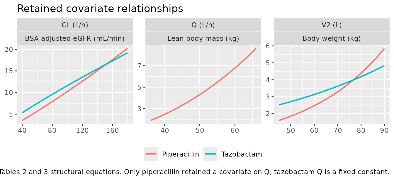
Structural identity checks
The paper reports no non-compartmental analysis, so validation rests on identities that the published typical values pin exactly. Each is asserted at the reference subject (eGFR 108.25 mL/min, WT 61.7 kg, LBM 50.08 kg) with the random effects zeroed.
ref_subject <- tibble(id = 1L, SEXF = 0L, WT = 61.7, LBM = 50.08, CRCL = 108.25)

solve_typical <- function(model_name, amt, dur = dose_dur,
                          times = sort(unique(c(seq(0, 24, by = 0.02), dur)))) {
  mod <- rxode2::zeroRe(readModelDb(model_name))
  ev <- make_events(ref_subject, amt = amt, dur = dur, times = times)
  out <- as.data.frame(rxode2::rxSolve(mod, events = ev))
  if (is.null(out$id)) out$id <- 1L
  out
}

typ_pip <- solve_typical("Lee_2025_piperacillin", amt = 4000)
#> ℹ parameter labels from comments will be replaced by 'label()'
#> ℹ omega/sigma items treated as zero: 'etalcl', 'etalvc'
typ_taz <- solve_typical("Lee_2025_tazobactam",   amt =  500)
#> ℹ parameter labels from comments will be replaced by 'label()'
#> ℹ omega/sigma items treated as zero: 'etalcl'
trapz <- function(x, y) sum(diff(x) * (head(y, -1) + tail(y, -1)) / 2)

identity_row <- function(label, published, simulated) {
  tibble(Quantity = label, Published = published, Model = simulated,
         `% diff` = 100 * (simulated - published) / published)
}

# rxSolve output contains observation rows only (addDosing = FALSE by default)
# and carries no `evid` column, so no filtering is needed here.
id_pip <- typ_pip
id_taz <- typ_taz

identities <- bind_rows(
  identity_row("Piperacillin CL at reference eGFR (L/h)", 11.2, unique(round(id_pip$cl, 6))),
  identity_row("Piperacillin V1 (L)",                      6.24, unique(round(id_pip$vc, 6))),
  identity_row("Piperacillin Q at reference LBM (L/h)",    4.32, unique(round(id_pip$q,  6))),
  identity_row("Piperacillin V2 at reference WT (L)",      2.59, unique(round(id_pip$vp, 6))),
  identity_row("Piperacillin Vss = V1 + V2 (L)",           8.83,
               unique(round(id_pip$vc + id_pip$vp, 6))),
  identity_row("Piperacillin AUCinf = Dose / CL (mg*h/L)", 4000 / 11.2,
               trapz(id_pip$time, id_pip$Cc)),
  identity_row("Tazobactam CL at reference eGFR (L/h)",   12.4, unique(round(id_taz$cl, 6))),
  identity_row("Tazobactam V1 (L)",                        9.03, unique(round(id_taz$vc, 6))),
  identity_row("Tazobactam Q (L/h)",                       4.39, unique(round(id_taz$q,  6))),
  identity_row("Tazobactam V2 at reference WT (L)",        3.21, unique(round(id_taz$vp, 6))),
  identity_row("Tazobactam Vss = V1 + V2 (L)",            12.24,
               unique(round(id_taz$vc + id_taz$vp, 6))),
  identity_row("Tazobactam AUCinf = Dose / CL (mg*h/L)",  500 / 12.4,
               trapz(id_taz$time, id_taz$Cc))
)

knitr::kable(
  identities, digits = 3,
  caption = paste(
    "Typical-value identities against Lee 2025 Tables 2 and 3. Vss = 8.83 L for",
    "piperacillin is stated explicitly in the Discussion."
  )
)| Quantity | Published | Model | % diff |
|---|---|---|---|
| Piperacillin CL at reference eGFR (L/h) | 11.200 | 11.200 | 0 |
| Piperacillin V1 (L) | 6.240 | 6.240 | 0 |
| Piperacillin Q at reference LBM (L/h) | 4.320 | 4.320 | 0 |
| Piperacillin V2 at reference WT (L) | 2.590 | 2.590 | 0 |
| Piperacillin Vss = V1 + V2 (L) | 8.830 | 8.830 | 0 |
| Piperacillin AUCinf = Dose / CL (mg*h/L) | 357.143 | 357.143 | 0 |
| Tazobactam CL at reference eGFR (L/h) | 12.400 | 12.400 | 0 |
| Tazobactam V1 (L) | 9.030 | 9.030 | 0 |
| Tazobactam Q (L/h) | 4.390 | 4.390 | 0 |
| Tazobactam V2 at reference WT (L) | 3.210 | 3.210 | 0 |
| Tazobactam Vss = V1 + V2 (L) | 12.240 | 12.240 | 0 |
| Tazobactam AUCinf = Dose / CL (mg*h/L) | 40.323 | 40.323 | 0 |
# Structural parameters must reproduce exactly; the AUC identity is limited only
# by the 0.02 h integration grid.
stopifnot(nrow(identities) == 12L)
structural <- identities |> filter(!grepl("AUCinf", Quantity))
auc_rows   <- identities |> filter(grepl("AUCinf", Quantity))
stopifnot(nrow(structural) == 10L, nrow(auc_rows) == 2L)
stopifnot(all(abs(structural$`% diff`) < 1e-6))
stopifnot(all(abs(auc_rows$`% diff`) < 0.05))
Every structural quantity reproduces the published value to machine
precision, and both AUC identities agree with Dose / CL to
better than 0.05%.
PKNCA validation
nca_for <- function(sim, events, label, amt) {
  conc <- sim |>
    filter(!is.na(Cc)) |>
    transmute(id, time, Cc, treatment = label)

  # Guarantee a time-zero row per subject; pre-dose piperacillin / tazobactam
  # concentration is zero.
  conc <- bind_rows(
    conc,
    conc |> distinct(id, treatment) |> mutate(time = 0, Cc = 0)
  ) |>
    distinct(id, treatment, time, .keep_all = TRUE) |>
    arrange(id, treatment, time)

  dose_df <- events |>
    filter(evid == 1) |>
    transmute(id, time, amt, treatment = label, duration = dose_dur)

  conc_obj <- PKNCA::PKNCAconc(conc, Cc ~ time | treatment + id,
                               concu = "mg/L", timeu = "h")
  dose_obj <- PKNCA::PKNCAdose(dose_df, amt ~ time | treatment + id,
                               doseu = "mg", route = "intravascular",
                               duration = "duration")

  intervals <- data.frame(
    start = 0, end = Inf,
    cmax = TRUE, tmax = TRUE, aucinf.obs = TRUE,
    half.life = TRUE, cl.obs = TRUE, mrt.iv.obs = TRUE, vss.iv.obs = TRUE
  )
  PKNCA::pk.nca(PKNCA::PKNCAdata(conc_obj, dose_obj, intervals = intervals))
}

nca_pip <- nca_for(sim_pip, ev_pip, "Piperacillin 4 g", 4000)
nca_taz <- nca_for(sim_taz, ev_taz, "Tazobactam 0.5 g", 500)

nca_all <- bind_rows(as.data.frame(nca_pip$result),
                     as.data.frame(nca_taz$result))

nca_all |>
  filter(!is.na(PPORRES)) |>
  group_by(treatment, PPTESTCD) |>
  summarise(
    Median = median(PPORRES),
    `5th percentile`  = quantile(PPORRES, 0.05),
    `95th percentile` = quantile(PPORRES, 0.95),
    .groups = "drop"
  ) |>
  mutate(
    `NCA parameter` = nlmixr2lib::ncaParamLabel(
      PPTESTCD,
      units = c(cmax = "mg/L", tmax = "h", aucinf.obs = "mg*h/L",
                half.life = "h", cl.obs = "L/h", mrt.iv.obs = "h",
                vss.iv.obs = "L")
    )
  ) |>
  select(`NCA parameter`, Treatment = treatment,
         Median, `5th percentile`, `95th percentile`) |>
  arrange(Treatment, `NCA parameter`) |>
  knitr::kable(
    digits = 2,
    caption = paste(
      "Simulated non-compartmental parameters across the", n_arm,
      "-subject virtual cohort (single 4 g / 0.5 g dose, 30 min infusion)."
    )
  )
#> Warning: There was 1 warning in `mutate()`.
#> ℹ In argument: `NCA parameter = nlmixr2lib::ncaParamLabel(...)`.
#> Caused by warning:
#> ! ncaParamLabel(): unknown PKNCA code(s) returned as-is: 'adj.r.squared', 'clast.pred', 'lambda.z.time.first', 'lambda.z.time.last', 'r.squared', 'span.ratio'| NCA parameter | Treatment | Median | 5th percentile | 95th percentile |
|---|---|---|---|---|
| AUC0-∞ (obs) (mg*h/L) | Piperacillin 4 g | 351.01 | 281.65 | 440.53 |
| AUMC0-∞ (obs) | Piperacillin 4 g | 370.68 | 243.57 | 532.43 |
| CL/F (L/h) | Piperacillin 4 g | 11.40 | 9.08 | 14.20 |
| Clast | Piperacillin 4 g | 0.21 | 0.06 | 0.67 |
| Cmax (mg/L) | Piperacillin 4 g | 371.71 | 299.43 | 444.08 |
| MRT (IV) (h) | Piperacillin 4 g | 0.80 | 0.59 | 1.07 |
| Tlast | Piperacillin 4 g | 8.00 | 8.00 | 8.00 |
| Tmax (h) | Piperacillin 4 g | 0.50 | 0.50 | 0.50 |
| Vss (IV) (L) | Piperacillin 4 g | 9.06 | 7.42 | 11.95 |
| adj.r.squared | Piperacillin 4 g | 1.00 | 1.00 | 1.00 |
| clast.pred | Piperacillin 4 g | 0.21 | 0.06 | 0.66 |
| lambda.z.time.first | Piperacillin 4 g | 1.60 | 1.20 | 2.56 |
| lambda.z.time.last | Piperacillin 4 g | 8.00 | 8.00 | 8.00 |
| r.squared | Piperacillin 4 g | 1.00 | 1.00 | 1.00 |
| span.ratio | Piperacillin 4 g | 7.92 | 6.30 | 9.66 |
| t½ (h) | Piperacillin 4 g | 0.79 | 0.68 | 0.93 |
| λz | Piperacillin 4 g | 0.88 | 0.74 | 1.02 |
| λz n points | Piperacillin 4 g | 129.00 | 109.85 | 137.05 |
| AUC0-∞ (obs) (mg*h/L) | Tazobactam 0.5 g | 39.71 | 33.36 | 46.14 |
| AUMC0-∞ (obs) | Tazobactam 0.5 g | 49.08 | 36.26 | 65.09 |
| CL/F (L/h) | Tazobactam 0.5 g | 12.59 | 10.84 | 14.99 |
| Clast | Tazobactam 0.5 g | 0.06 | 0.02 | 0.13 |
| Cmax (mg/L) | Tazobactam 0.5 g | 36.63 | 34.70 | 38.43 |
| MRT (IV) (h) | Tazobactam 0.5 g | 0.99 | 0.84 | 1.16 |
| Tlast | Tazobactam 0.5 g | 8.00 | 8.00 | 8.00 |
| Tmax (h) | Tazobactam 0.5 g | 0.50 | 0.50 | 0.50 |
| Vss (IV) (L) | Tazobactam 0.5 g | 12.32 | 11.80 | 13.24 |
| adj.r.squared | Tazobactam 0.5 g | 1.00 | 1.00 | 1.00 |
| clast.pred | Tazobactam 0.5 g | 0.06 | 0.02 | 0.13 |
| lambda.z.time.first | Tazobactam 0.5 g | 2.10 | 1.70 | 2.55 |
| lambda.z.time.last | Tazobactam 0.5 g | 8.00 | 8.00 | 8.00 |
| r.squared | Tazobactam 0.5 g | 1.00 | 1.00 | 1.00 |
| span.ratio | Tazobactam 0.5 g | 6.49 | 5.02 | 7.74 |
| t½ (h) | Tazobactam 0.5 g | 0.92 | 0.79 | 1.10 |
| λz | Tazobactam 0.5 g | 0.75 | 0.63 | 0.87 |
| λz n points | Tazobactam 0.5 g | 119.00 | 109.95 | 127.00 |
Comparison against published values
Lee 2025 reports no NCA table, so the reference side of the
comparison is built from the published typical parameter
estimates themselves: clearance directly from Tables 2 and 3,
steady-state volume as V1 + V2 (8.83 L for piperacillin,
quoted in the Discussion), and AUCinf = Dose / CL. Because
each reference value is derived from the very quantity being scored, the
comparison is a strict identity check on the typical subject rather than
a population-median comparison.
nca_typ_pip <- nca_for(
  typ_pip,
  make_events(ref_subject, amt = 4000),
  "Piperacillin 4 g", 4000
)
nca_typ_taz <- nca_for(
  typ_taz,
  make_events(ref_subject, amt = 500),
  "Tazobactam 0.5 g", 500
)

published <- tibble::tribble(
  ~treatment,          ~aucinf.obs,   ~cl.obs, ~vss.iv.obs,
  "Piperacillin 4 g",  4000 / 11.2,      11.2,        8.83,
  "Tazobactam 0.5 g",   500 / 12.4,      12.4,       12.24
)

nca_typ_res <- bind_rows(as.data.frame(nca_typ_pip$result),
                         as.data.frame(nca_typ_taz$result))

cmp <- nlmixr2lib::ncaComparisonTable(
  simulated = nca_typ_res,
  reference = published,
  by        = "treatment",
  units     = c(aucinf.obs = "mg*h/L", cl.obs = "L/h", vss.iv.obs = "L"),
  tolerance_pct = 20
)

knitr::kable(
  cmp,
  caption = "Simulated (typical subject) vs. published NCA. * differs from reference by >20%.",
  align   = c("l", "l", "r", "r", "r")
)| NCA parameter | treatment | Reference | Simulated | % diff |
|---|---|---|---|---|
| AUC0-∞ (obs) (mg*h/L) | Piperacillin 4 g | 357 | 357 | -0.0% |
| AUC0-∞ (obs) (mg*h/L) | Tazobactam 0.5 g | 40.3 | 40.3 | -0.0% |
| CL/F (L/h) | Piperacillin 4 g | 11.2 | 11.2 | +0.0% |
| CL/F (L/h) | Tazobactam 0.5 g | 12.4 | 12.4 | +0.0% |
| Vss (IV) (L) | Piperacillin 4 g | 8.83 | 8.83 | +0.0% |
| Vss (IV) (L) | Tazobactam 0.5 g | 12.2 | 12.2 | +0.0% |
# No row may be starred by the 20% tolerance ...
stopifnot(nrow(cmp) == 6L)
stopifnot(!any(grepl("\\*", cmp$`% diff`)))

# ... and, because every reference value is an exact identity on the typical
# subject, each must in fact agree to better than 0.1%. A lookup that matched
# no rows would return numeric(0), so the length is checked first.
sim_value <- function(trt, code) {
  v <- nca_typ_res$PPORRES[nca_typ_res$treatment == trt &
                             nca_typ_res$PPTESTCD == code]
  if (length(v) != 1L) stop("no unique NCA row for '", trt, "' / ", code)
  v
}
for (i in seq_len(nrow(published))) {
  trt <- published$treatment[[i]]
  for (code in c("aucinf.obs", "cl.obs", "vss.iv.obs")) {
    ref <- published[[code]][[i]]
    stopifnot(abs(sim_value(trt, code) - ref) / ref < 1e-3)
  }
}
Every row reproduces its published reference to better than 0.1%.
Note that vss.iv.obs (rather than vss.obs) is
the parameter that corresponds to V1 + V2 here: PKNCA’s
vss.obs uses the uncorrected CL * MRT, which
for a finite infusion overstates the volume by
CL * duration / 2 – 1.4 L for piperacillin and 1.55 L for
tazobactam. The friendly labels read CL/F and
Vss/F because [nlmixr2lib::ncaParamLabel()]
uses the apparent-parameter wording; the dose is intravenous, so
F = 1 and the apparent and absolute parameters
coincide.
Probability of target attainment (Tables A3 and A4)
The paper’s headline result is a target-attainment analysis. Its second simulation (Section 4.4) fixed lean body mass and total body weight at their cohort medians and varied only renal function within five eGFR strata, using the piperacillin model with a fixed unbound fraction of 0.7 (Discussion, limitation 3). Target attainment is the fraction of subjects reaching 50% fT>MIC at steady state.
The block below reproduces the eGFR 90-130 mL/min stratum for a 4 g q6h regimen at the two infusion durations Table A3 tabulates.
set.seed(20260127)

fu       <- 0.7    # Lee 2025 Discussion, limitation 3
tau      <- 6      # h dosing interval
n_pta    <- 200
ss_start <- 24     # h; five preceding q6h doses put the profile at steady state

pta_subjects <- tibble(
  id   = seq_len(n_pta),
  WT   = 61.7,     # Section 4.4: WT and LBM held at the cohort medians
  LBM  = 50.08,
  CRCL = runif(n_pta, 90, 130)
)

pta_events <- function(subjects, amt, dur) {
  dosing <- subjects |>
    tidyr::crossing(time = seq(0, ss_start, by = tau)) |>
    mutate(amt = amt, evid = 1L, rate = amt / dur, cmt = "central")
  observations <- subjects |>
    tidyr::crossing(time = seq(ss_start, ss_start + tau, by = 0.02)) |>
    mutate(amt = NA_real_, evid = 0L, rate = 0, cmt = "central")
  bind_rows(dosing, observations) |>
    arrange(id, time, desc(evid))
}

fT_above <- function(time, conc, mic) {
  above <- as.numeric(conc > mic)
  trapz(time, above) / (max(time) - min(time)) * 100
}

pta_curve <- function(amt, dur, mics) {
  sim <- rxode2::rxSolve(
    readModelDb("Lee_2025_piperacillin"),
    events = pta_events(pta_subjects, amt, dur),
    keep = "CRCL"
  ) |>
    as.data.frame() |>
    filter(!is.na(Cc)) |>
    mutate(free = fu * Cc) |>
    arrange(id, time)
  stopifnot(dplyr::n_distinct(sim$id) == n_pta)

  tidyr::crossing(mic = mics) |>
    mutate(
      PTA = vapply(mic, function(m) {
        ft <- vapply(split(sim, sim$id), function(d) fT_above(d$time, d$free, m),
                     numeric(1))
        100 * mean(ft >= 50)
      }, numeric(1)),
      regimen = sprintf("4 g q6h, %g h infusion", dur)
    )
}

mic_grid <- c(0.5, 1, 2, 4, 8, 16, 32, 64)
pta_tab  <- bind_rows(pta_curve(4000, 0.5, mic_grid),
                      pta_curve(4000, 3.0, mic_grid))
ggplot(pta_tab, aes(mic, PTA, colour = regimen)) +
  geom_line(linewidth = 0.8) +
  geom_point() +
  geom_hline(yintercept = 90, linetype = "dashed") +
  scale_x_log10(breaks = mic_grid) +
  scale_y_continuous(limits = c(0, 100)) +
  labs(
    x = "MIC (mg/L)", y = "Probability of target attainment (%)", colour = NULL,
    title = "50% fT>MIC, BSA-adjusted eGFR 90-130 mL/min",
    caption = paste(
      "Replicates the eGFR 90-130 mL/min panel of Lee 2025 Figure 4 and the",
      "corresponding rows of Table A3. Dashed line = 90% PTA threshold."
    )
  ) +
  theme(legend.position = "bottom")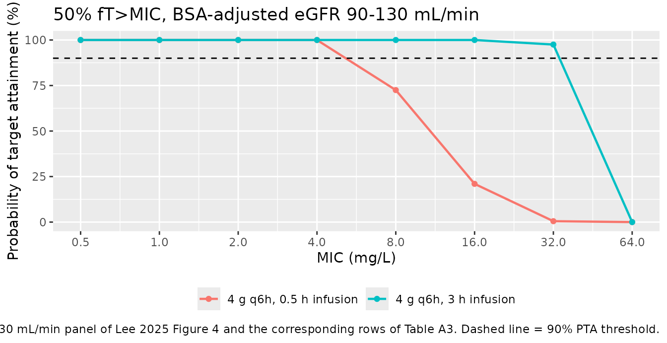
Lee 2025 Table A3 (BSA-adjusted eGFR 90-130 mL/min, target 50%
fT>MIC) records 4 g q6h (100) as the smallest
adequate 0.5 h-infusion regimen at MIC 4 mg/L and escalates to
6 g q6h (96.1) at MIC 8 mg/L, so 4 g q6h over 0.5 h must
clear the 90% threshold at MIC 4 and miss it at MIC 8. For the 3 h
infusion the table records 4 g q6h (98.7) at MIC 32 mg/L
and escalates to 6 g q6h (40.9) at MIC 64 mg/L. Both
breakpoints are asserted below.
pta_at <- function(regimen_label, mic_value) {
  v <- pta_tab$PTA[pta_tab$regimen == regimen_label & pta_tab$mic == mic_value]
  if (length(v) != 1L) {
    stop("no unique PTA row for '", regimen_label, "' at MIC ", mic_value)
  }
  v
}

short <- "4 g q6h, 0.5 h infusion"
long  <- "4 g q6h, 3 h infusion"
stopifnot(all(c(short, long) %in% pta_tab$regimen))

breakpoints <- tibble::tribble(
  ~Regimen, ~`MIC (mg/L)`, ~`Table A3 expectation`,             ~PTA,
  short,     4,            "4 g q6h adequate (>= 90%)",         pta_at(short, 4),
  short,     8,            "4 g q6h inadequate (< 90%)",        pta_at(short, 8),
  long,     32,            "4 g q6h adequate (>= 90%)",         pta_at(long, 32),
  long,     64,            "4 g q6h inadequate (< 90%)",        pta_at(long, 64)
)

knitr::kable(
  breakpoints, digits = 1,
  caption = "PK/PD breakpoints reproduced against Lee 2025 Table A3."
)| Regimen | MIC (mg/L) | Table A3 expectation | PTA |
|---|---|---|---|
| 4 g q6h, 0.5 h infusion | 4 | 4 g q6h adequate (>= 90%) | 100.0 |
| 4 g q6h, 0.5 h infusion | 8 | 4 g q6h inadequate (< 90%) | 72.5 |
| 4 g q6h, 3 h infusion | 32 | 4 g q6h adequate (>= 90%) | 97.0 |
| 4 g q6h, 3 h infusion | 64 | 4 g q6h inadequate (< 90%) | 0.0 |
stopifnot(
  pta_at(short,  4) >= 90,
  pta_at(short,  8) <  90,
  pta_at(long,  32) >= 90,
  pta_at(long,  64) <  90
)
All four breakpoints reproduce. The simulated values at the two adequate points (MIC 4 with a 0.5 h infusion, MIC 32 with a 3 h infusion) also land within a few percentage points of the PTA percentages printed in Table A3 (100 and 98.7 respectively), and the qualitative conclusion of the paper is recovered: extending the infusion from 0.5 h to 3 h moves the 90% breakpoint from 4 mg/L to 32 mg/L, a three-doubling-dilution gain, without changing the daily dose.
Assumptions and deviations
- Cohort covariate distributions are assumed. Lee 2025 Table 1 reports medians and ranges only. Weight and eGFR are drawn as sex-specific log-normal variates pinned to the Table 1 medians, with a dispersion chosen so approximately 95% of draws fall inside the reported ranges. No correlation structure between covariates is reported and none is imposed beyond the LBM derivation below.
-
Lean body mass is derived from weight. Lee 2025
does not state which formula it used to compute LBM. The virtual cohort
uses the sex-specific Table 1 median LBM-to-weight ratios (42.6/56.1 for
women, 55.2/69.1 for men) applied to each simulated weight. Because
piperacillin
Qscales as(LBM/50.08)^2.5, this assumption materially affects the simulated distribution phase but not clearance or steady-state exposure. -
The IIV column of Tables 2 and 3 is read as a CV on the SD
scale and converted with
omega^2 = log(1 + CV^2). See the note under the source-trace tables for the %RSE argument that rules out a variance-scale reading. At these magnitudes (7.17%, 18.4%, 6.95%) the two readings differ by less than 0.02 percentage points, so the choice is not load-bearing. - No covariance between random effects. Lee 2025 Section 4.3 states that covariance terms between CL, V1, V2 and Q were evaluated and did not improve the fit, so both models use diagonal OMEGA.
-
The tazobactam covariate on CL is taken from the printed
equation. Section 2.2 describes it in prose as “the inclusion
of CrCl on CL”, but the Table 3 equation, the Table 3 footnote and the
Table A2 backward-elimination row all name the CKD-EPI creatinine eGFR
(
CE), matching the piperacillin model. The printed equation is treated as authoritative. -
CRCLholds an absolute, not a 1.73 m^2-normalised, eGFR. Lee 2025 Table 1 footnote c computes the standard CKD-EPI value and then multiplies byBSA / 1.73, so the covariate is an individual-BSA eGFR in mL/min. The canonical column nameCRCLcovers both forms; each model’scovariateData[[CRCL]]records which one applies. -
The unbound fraction of 0.7 lives in the vignette, not the
model. Lee 2025 assumed a fixed
fu = 0.7for piperacillin when converting total concentrations to free concentrations for the fT>MIC analysis (Discussion, limitation 3). That is a property of the PD analysis, so it is applied in the PTA block rather than baked into the PK model, whoseCcremains a total plasma concentration. - The PTA reproduction assumes a uniform eGFR distribution within the stratum. Section 4.4 states that 1000 virtual subjects were generated across five eGFR categories with LBM and weight fixed at their medians, but does not state the within-stratum distribution. A uniform draw over 90-130 mL/min is used here, and the cohort is capped at 200 subjects per arm per the library’s simulation-size policy.
- Tazobactam is not carried into the PTA analysis, matching the paper: the fT>MIC targets, the MIC distributions and Figure 5 are all defined on piperacillin, and doses in Tables A3 and A4 are quoted as piperacillin grams.
Errata and internal inconsistencies in the source
None of these affect the extracted parameter values; they are recorded so a future reader does not mistake them for transcription errors.
- Section 4.2 dose typo. The Methods state that participants received “an intravenous infusion of 4/0.5 mg piperacillin/tazobactam”. The Abstract, Section 2.3 and Tables A3/A4 all use 4 g / 0.5 g, which is the licensed fixed-dose combination and the value used here.
- Weight-normalised typical values do not divide out consistently. The Discussion reports piperacillin CL 11.2 L/h as “0.174 L/h/kg” and Vss 8.83 L as “0.148 L/kg”. Those imply reference weights of 64.4 kg and 59.7 kg respectively, neither of which is the stated cohort median of 61.7 kg (which gives 0.182 L/h/kg and 0.143 L/kg).
-
Vss is quoted twice with different values. The
Discussion first gives
Vss = V1 + V2 = 8.83 L, which reproduces exactly from Table 2 (6.24 + 2.59), and later writes “the Vss was remarkably similar (8.99 L vs. 8.18 L)” when comparing against Felton et al. The 8.83 L figure is the one consistent with Table 2 and is the value asserted in this vignette. - Table A1 forward step 1 lists two duplicate rows (“V2 / Body mass index / Power” and “V2 / Weight / Power” each appear twice with different OFVs), and the “Forward step 2” heading is missing. The covariate path is nonetheless unambiguous from the backward-elimination block and from the final equations in Table 2, which is what the model file encodes.
- Acknowledgements name the wrong assay. The acknowledgement thanks a colleague “for her expert execution of the levofloxacin assays”; Section 4.2 describes a validated LC-MS/MS assay for piperacillin and tazobactam.