Methotrexate (Zhang 2015)
Source:vignettes/articles/Zhang_2015_methotrexate.Rmd
Zhang_2015_methotrexate.RmdModel and source
- Citation: Zhang W, Zhang Q, Tian X, Zhao H, Lu W, Zhen J, Niu X. (2015). Population Pharmacokinetics of High-dose Methotrexate After Intravenous Administration in Chinese Osteosarcoma Patients from a Single Institution. Chin Med J (Engl) 128(1):111-118. doi:10.4103/0366-6999.147829.
- Description: Two-compartment population PK model for intravenous high-dose methotrexate (8-12 g/m^2 infused over 4-6 h) in Chinese osteosarcoma patients at a single Beijing institution; central clearance carries a linear effect of the number of prior methotrexate chemotherapy cycles and of pre-dose creatinine clearance, and intercompartmental clearance and peripheral volume each carry a linear effect of body surface area (Zhang 2015)
- Article: Chin Med J (Engl) 2015;128(1):111-118 (open access via PMC4837805)
Zhang 2015 is a two-compartment population PK analysis of high-dose methotrexate (HD-MTX) given as a 4-6 h intravenous infusion to Chinese osteosarcoma patients at Beijing Jishuitan Hospital. It is, by the authors’ account, the first NONMEM population analysis of HD-MTX in a Chinese osteosarcoma cohort.
Read the “Assumptions, deviations and errata” section before using this model. Three of the four covariate-effect signs printed in the source paper have been corrected during extraction, and the creatinine-clearance covariate must be supplied on the paper’s own numeric scale rather than in mL/min.
Population
148 patients with osteosarcoma contributed 274 HD-MTX courses between August 2009 and August 2010 (Zhang 2015 Methods, “Subjects”). Age was 17.00 +/- 7.06 years (Table 1 median 17, range 6-49), height 166.00 +/- 12.44 cm, body weight 58.00 +/- 18.28 kg (Table 1 median 58, range 20-97) and body surface area 1.63 +/- 0.27 m^2 (Table 1 median 1.63, range 0.62-2.21). 194 of the 274 courses were in males and 80 in females, i.e. 29% female. The cohort therefore spans children through middle-aged adults, which is why the BSA range reaches down to 0.62 m^2.
Methotrexate 8-12 g/m^2 was infused over 4-6 h in darkness, embedded in a protocolized regimen of hyperhydration and urine alkalinization, with vincristine and tropisetron, oral sodium bicarbonate and allopurinol. Leucovorin rescue 12 mg every 6 h began 6-8 h after the end of the infusion and continued until plasma methotrexate fell below 0.05 umol/L. Plasma was sampled at 0, 6, 12, 24, 48 and 72 h after the start of the infusion, with additional 24-hourly samples until the concentration fell below 0.05 umol/L, and assayed by fluorescence polarization immunoassay (quantification limit 0.01 umol/L).
One structural feature of the analysis matters for interpreting every variance in this model. Repeat courses in the same patient were treated as independent individuals during model building; Zhang 2015 says so explicitly in the Discussion (“we treated them as totally separate individuals in the modeling process to gather more data, but that also meant that we ignored the internal correlation within patients”). The reported inter-individual variances are therefore between-course variances that confound inter-individual with between-occasion variability, over 274 courses rather than 148 subjects.
The same information is available programmatically via the model’s
population metadata
(readModelDb("Zhang_2015_methotrexate")()$population).
Source trace
The per-parameter origin is recorded as an in-file comment next to
each ini() entry in
inst/modeldb/specificDrugs/Zhang_2015_methotrexate.R. The
table below collects them in one place for review.
| Equation / parameter | Value | Source location |
|---|---|---|
lcl (CL1) |
6.20 L/h (RSE 4.87%) | Table 2, final model standard value |
lvc (V1) |
19.6 L (RSE 4.39%) | Table 2, final model standard value |
lq (CL2) |
0.0172 L/h (RSE 14.9%) | Table 2, final model standard value |
lvp (V2) |
0.515 L (RSE 9.92%) | Table 2, final model standard value |
e_cycle_cl |
0.0183 (RSE 35.6%) | Table 2, theta CL1-MTXNUM
|
e_crcl_cl |
0.0416 (RSE 32.2%) | Table 2, theta CL1-CrCl
|
e_bsa_q |
0.880 (RSE 28.3%) | Table 2, theta CL2-BODYAREA
|
e_bsa_vp |
0.874 (RSE 21.2%) | Table 2, theta V2-BODYAREA
|
| CRCL centering | 1.89 | Final-model equation, Results |
| BSA centering | 1.62 m^2 | Final-model equations, Results |
etalcl |
0.00719 = 0.0848^2 | Table 2, inter-individual RSD 8.48% on CL1 |
etalq |
0.259 = 0.509^2 | Table 2, inter-individual RSD 50.9% on CL2 |
etalvp |
0.153 = 0.391^2 | Table 2, inter-individual RSD 39.1% on V2 |
| V1 inter-individual variability | not estimated | Table 2 leaves the cell blank in base and final models; Abstract calls it “extremely small” |
| Covariate model form | P = P_tv * [1 +/- theta * (cov - mean)] |
Methods, “Fixed effect model”; Results, final-model equations |
| Random-effect form | P_ij = P_TVj * exp(eta_ij) |
Methods, “Statistical model” |
| Residual-error form | C_obs = C_pred * (1 + eps1) + eps2 |
Methods, “Residual random effect model”; magnitudes never reported |
| Two-compartment IV disposition | n/a | Results, “Base model”; Table 2 parameterization CL1 / V1 / CL2 / V2 |
| CL2 is intercompartmental | n/a | Discussion, comparing “intercompartmental clearance (0.0172 L/h)” with Aquerreta’s CLD1 |
Virtual cohort
Original observed data are not publicly available. The cohort below draws covariates from the marginal distributions reported in Zhang 2015 Table 1 and the Subjects section.
# `set.seed()` seeds R's RNG. It does NOT seed rxode2's simulation RNG, and
# rxode2's streams are partitioned PER SOLVER THREAD -- so this cohort is
# reproducible on this machine and different on a machine with a different
# thread count. Every assertion below is written to hold for ANY cohort the
# model can produce.
set.seed(20150105)

n_per_arm <- 150L

# Methotrexate molar mass, used only to convert the paper's g/m^2 prescription
# into the umol amount unit the model is built in. This is a physical constant
# (C20H22N8O5), not a value from Zhang 2015.
MW_MTX <- 454.44  # g/mol

# Truncated sampler matching a reported median and observed range.
rtrunc_lnorm <- function(n, med, lo, hi, sdlog) {
  x <- stats::rlnorm(n, meanlog = log(med), sdlog = sdlog)
  pmin(pmax(x, lo), hi)
}
rtrunc_norm <- function(n, mean, sd, lo, hi) {
  pmin(pmax(stats::rnorm(n, mean, sd), lo), hi)
}

make_cohort <- function(n, dose_g_m2, arm, id_offset = 0L) {
  subj <- tibble(
    id    = id_offset + seq_len(n),
    arm   = arm,
    # BSA: Subjects section 1.63 +/- 0.27 m^2; Table 1 range 0.62-2.21.
    BSA   = rtrunc_norm(n, 1.63, 0.27, 0.62, 2.21),
    # CRCL on the SOURCE'S OWN numeric scale: Table 1 median 1.88, range
    # 0.94-4.64 (see the units note in "Assumptions, deviations and errata").
    CRCL  = rtrunc_lnorm(n, 1.88, 0.94, 4.64, sdlog = 0.35),
    # CYCLE (source MTXNUM): Table 1 median 2, range 1-12, right-skewed.
    CYCLE = pmin(1L + stats::rpois(n, 1.4), 12L)
  ) |>
    mutate(
      dose_g   = dose_g_m2 * BSA,
      dose_umol = dose_g / MW_MTX * 1e6,
      # Methods: 4-6 h infusion. The paper does not report the distribution of
      # actual durations, so 6 h (the upper end) is used throughout.
      dur_h    = 6
    )

  dosing <- subj |>
    mutate(time = 0, evid = 1L, cmt = "central",
           amt = dose_umol, rate = dose_umol / dur_h)

  # Observation grid: dense through the distribution phase, out to 144 h so the
  # terminal phase is resolved. Observations are placed on the ODE STATE
  # `central`; rxode2 returns the algebraic observable `Cc` as a column there.
  tgrid <- c(seq(0, 12, by = 0.25), seq(12.5, 36, by = 0.5), seq(37, 144, by = 1))
  obs <- subj |>
    tidyr::crossing(time = tgrid) |>
    mutate(evid = 0L, cmt = "central", amt = NA_real_, rate = NA_real_)

  bind_rows(dosing, obs) |>
    arrange(id, time, desc(evid)) |>
    select(id, arm, time, evid, cmt, amt, rate, BSA, CRCL, CYCLE, dose_g, dose_umol, dur_h)
}

events <- bind_rows(
  make_cohort(n_per_arm,  8, "8 g/m2",  id_offset =              0L),
  make_cohort(n_per_arm, 10, "10 g/m2", id_offset =      n_per_arm),
  make_cohort(n_per_arm, 12, "12 g/m2", id_offset = 2L * n_per_arm)
)

# Disjoint IDs across arms are mandatory -- duplicates silently merge into one
# subject receiving the summed dose.
stopifnot(!anyDuplicated(unique(events[, c("id", "time", "evid")])))
stopifnot(length(unique(events$id)) == 3L * n_per_arm)

events |>
  filter(evid == 1) |>
  group_by(arm) |>
  summarise(
    n = n(),
    `BSA median (m^2)`  = round(median(BSA), 2),
    `CRCL median`       = round(median(CRCL), 2),
    `CYCLE median`      = median(CYCLE),
    `Dose median (g)`   = round(median(dose_g), 1),
    .groups = "drop"
  ) |>
knitr::kable(caption = "Virtual cohort by dose arm (150 subjects per arm).")| arm | n | BSA median (m^2) | CRCL median | CYCLE median | Dose median (g) |
|---|---|---|---|---|---|
| 10 g/m2 | 150 | 1.65 | 1.80 | 2 | 16.5 |
| 12 g/m2 | 150 | 1.64 | 1.81 | 2 | 19.7 |
| 8 g/m2 | 150 | 1.67 | 1.88 | 2 | 13.4 |
Simulation
mod <- readModelDb("Zhang_2015_methotrexate")

sim <- rxode2::rxSolve(
  mod,
  events = events,
  keep   = c("arm", "BSA", "CRCL", "CYCLE", "dose_umol", "dur_h")
) |>
  as.data.frame()
#> ℹ parameter labels from comments will be replaced by 'label()'

# Every individual parameter must be strictly positive: the covariate model is
# LINEAR, so a sufficiently extreme covariate would drive a multiplier through
# zero. Within the observed covariate ranges it cannot, and this guard proves it
# for the drawn cohort.
stopifnot(all(sim$cl > 0), all(sim$vc > 0), all(sim$q > 0), all(sim$vp > 0))
# The far tail decays through several orders of magnitude, where the solver can
# return a vanishingly small negative value; allow for that rather than asserting
# an exact zero floor.
stopifnot(all(is.finite(sim$Cc)), all(sim$Cc > -1e-6))
Figure 1 – concentration-time profiles on a log scale
# Replicates Figure 1 of Zhang 2015 (log concentration versus time after the
# start of the intravenous methotrexate infusion).
sim |>
  filter(Cc > 0, time <= 96) |>
  group_by(arm, time) |>
  summarise(
    Q05 = quantile(Cc, 0.05),
    Q50 = quantile(Cc, 0.50),
    Q95 = quantile(Cc, 0.95),
    .groups = "drop"
  ) |>
  ggplot(aes(time, Q50)) +
  geom_ribbon(aes(ymin = Q05, ymax = Q95), alpha = 0.25) +
  geom_line() +
  facet_wrap(~arm) +
  scale_y_log10() +
  scale_x_continuous(breaks = c(0, 24, 48, 72, 96)) +
  labs(
    x = "Time after start of infusion (h)",
    y = "Plasma methotrexate (umol/L)",
    title = "Figure 1 -- simulated HD-MTX concentration-time profiles",
    caption = "Median and 5th-95th percentile. Replicates Figure 1 of Zhang 2015."
  )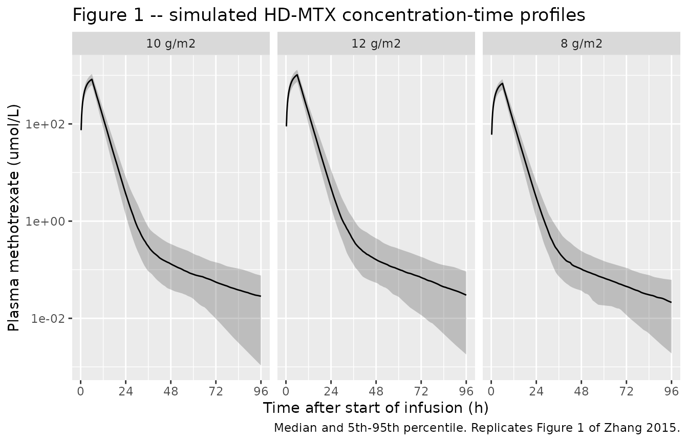
The paper’s Figure 1 is a scatter of all 274 courses without a fitted overlay, so this is a distributional rather than a point-by-point replication: the comparable features are the 2-3 orders of magnitude drop over the first 24 h and the shallow terminal phase thereafter.
Covariate-model verification
This is the most important check in this vignette, because it gates
the sign correction described in the errata. Each individual parameter
returned by rxSolve is compared against the published
final-model equations evaluated by hand. Both sides use the same
parameter values, so the difference is pure floating-point arithmetic
and a tight bound is the correct assertion.
typ <- rxode2::rxSolve(
  rxode2::zeroRe(mod),
  events = events,
  keep   = c("arm", "BSA", "CRCL", "CYCLE")
) |>
  as.data.frame() |>
  distinct(id, .keep_all = TRUE)
#> ℹ parameter labels from comments will be replaced by 'label()'
#> ℹ omega/sigma items treated as zero: 'etalcl', 'etalq', 'etalvp'
#> Warning: multi-subject simulation without without 'omega'

# Zhang 2015 final-model equations, as corrected (see errata). Coefficients are
# transcribed independently here from Table 2 so a transcription slip in the
# model file shows up as a mismatch rather than cancelling out.
expected <- typ |>
  mutate(
    cl_expected = 6.20   * (1 - 0.0183 * CYCLE) * (1 + 0.0416 * (CRCL - 1.89)),
    vc_expected = 19.6,
    q_expected  = 0.0172 * (1 + 0.880 * (BSA - 1.62)),
    vp_expected = 0.515  * (1 + 0.874 * (BSA - 1.62))
  )

rel_err <- with(expected, c(
  cl = max(abs(cl / cl_expected - 1)),
  vc = max(abs(vc / vc_expected - 1)),
  q  = max(abs(q  / q_expected  - 1)),
  vp = max(abs(vp / vp_expected - 1))
))

tibble(
  Parameter = c("CL1", "V1", "CL2", "V2"),
  `Max relative error vs published equation` = sprintf("%.2e", rel_err)
) |>
knitr::kable(caption = "Individual parameters reproduce the published final-model equations exactly.")| Parameter | Max relative error vs published equation |
|---|---|
| CL1 | 4.44e-15 |
| V1 | 1.67e-15 |
| CL2 | 3.33e-16 |
| V2 | 4.44e-16 |
# Deterministic identity, not a simulated statistic: machine precision applies.
stopifnot(all(rel_err < 1e-10))
Direction of each covariate effect
The four directions below are the ones Zhang 2015 states in words in its Discussion. They are asserted on typical values, which are deterministic, so exact comparisons are appropriate here (unlike assertions on a random cohort).
probe <- function(CYCLE, CRCL, BSA) {
  ev <- rxode2::et(amt = 3.6e4, rate = 6e3, cmt = "central") |>
    rxode2::et(c(0, 24), cmt = "central")
  ev <- as.data.frame(ev)
  ev$CYCLE <- CYCLE; ev$CRCL <- CRCL; ev$BSA <- BSA
  s <- rxode2::rxSolve(rxode2::zeroRe(mod), ev, returnType = "data.frame")
  c(cl = s$cl[1], q = s$q[1], vp = s$vp[1])
}

lo_cycle <- probe(CYCLE = 1,  CRCL = 1.88, BSA = 1.63)
#> ℹ parameter labels from comments will be replaced by 'label()'
#> ℹ omega/sigma items treated as zero: 'etalcl', 'etalq', 'etalvp'
hi_cycle <- probe(CYCLE = 12, CRCL = 1.88, BSA = 1.63)
#> ℹ parameter labels from comments will be replaced by 'label()'
#> ℹ omega/sigma items treated as zero: 'etalcl', 'etalq', 'etalvp'
lo_crcl  <- probe(CYCLE = 2,  CRCL = 0.94, BSA = 1.63)
#> ℹ parameter labels from comments will be replaced by 'label()'
#> ℹ omega/sigma items treated as zero: 'etalcl', 'etalq', 'etalvp'
hi_crcl  <- probe(CYCLE = 2,  CRCL = 4.64, BSA = 1.63)
#> ℹ parameter labels from comments will be replaced by 'label()'
#> ℹ omega/sigma items treated as zero: 'etalcl', 'etalq', 'etalvp'
lo_bsa   <- probe(CYCLE = 2,  CRCL = 1.88, BSA = 0.62)
#> ℹ parameter labels from comments will be replaced by 'label()'
#> ℹ omega/sigma items treated as zero: 'etalcl', 'etalq', 'etalvp'
hi_bsa   <- probe(CYCLE = 2,  CRCL = 1.88, BSA = 2.21)
#> ℹ parameter labels from comments will be replaced by 'label()'
#> ℹ omega/sigma items treated as zero: 'etalcl', 'etalq', 'etalvp'

directions <- tibble::tribble(
  ~`Published claim (Zhang 2015 Discussion)`,                    ~`Low covariate`,      ~`High covariate`,     ~Holds,
  "CL1 decreases as the MTX course number rises",                lo_cycle[["cl"]],      hi_cycle[["cl"]],      hi_cycle[["cl"]] < lo_cycle[["cl"]],
  "CL1 decreases as creatinine clearance falls",                 lo_crcl[["cl"]],       hi_crcl[["cl"]],       hi_crcl[["cl"]]  > lo_crcl[["cl"]],
  "CL2 correlates positively with body surface area",            lo_bsa[["q"]],         hi_bsa[["q"]],         hi_bsa[["q"]]    > lo_bsa[["q"]],
  "V2 correlates positively with body surface area",             lo_bsa[["vp"]],        hi_bsa[["vp"]],        hi_bsa[["vp"]]   > lo_bsa[["vp"]]
)

directions |>
  mutate(across(c(`Low covariate`, `High covariate`), ~signif(.x, 4))) |>
knitr::kable(caption = "Each retained covariate moves its parameter in the direction the paper states in prose.")| Published claim (Zhang 2015 Discussion) | Low covariate | High covariate | Holds |
|---|---|---|---|
| CL1 decreases as the MTX course number rises | 6.084000 | 4.83600 | TRUE |
| CL1 decreases as creatinine clearance falls | 5.737000 | 6.65600 | TRUE |
| CL2 correlates positively with body surface area | 0.002064 | 0.02613 | TRUE |
| V2 correlates positively with body surface area | 0.064890 | 0.78060 | TRUE |
All four hold. Under the signs as literally printed in the paper’s final-model equations, the last three rows would all reverse, which is the evidence that led to the correction documented in the errata.
PKNCA validation
sim_nca <- sim |>
  filter(!is.na(Cc)) |>
  select(id, time, Cc, arm)

# Guarantee a time = 0 record per subject; for an infusion beginning at t = 0
# the pre-dose concentration is 0.
sim_nca <- bind_rows(
  sim_nca,
  sim_nca |> distinct(id, arm) |> mutate(time = 0, Cc = 0)
) |>
  distinct(id, arm, time, .keep_all = TRUE) |>
  arrange(id, time)

conc_obj <- PKNCA::PKNCAconc(sim_nca, Cc ~ time | arm + id,
                             concu = "umol/L", timeu = "h")

dose_df <- events |>
  filter(evid == 1) |>
  select(id, time, amt, arm)

dose_obj <- PKNCA::PKNCAdose(dose_df, amt ~ time | arm + id, doseu = "umol")

intervals <- data.frame(
  start       = 0,
  end         = Inf,
  cmax        = TRUE,
  tmax        = TRUE,
  auclast     = TRUE,
  aucinf.obs  = TRUE,
  half.life   = TRUE,
  clast.obs   = TRUE
)

nca_res <- PKNCA::pk.nca(PKNCA::PKNCAdata(conc_obj, dose_obj, intervals = intervals))

nca_wide <- as.data.frame(nca_res) |>
  select(arm, id, PPTESTCD, PPORRES) |>
  tidyr::pivot_wider(names_from = PPTESTCD, values_from = PPORRES)

# A gate that cannot go red is worse than no gate: confirm rows exist first.
stopifnot(nrow(nca_wide) == 3L * n_per_arm, !anyNA(nca_wide$aucinf.obs))

nca_wide |>
  group_by(arm) |>
  summarise(
    `Cmax (umol/L)`      = median(cmax),
    `Tmax (h)`           = median(tmax),
    `AUCinf (umol*h/L)`  = median(aucinf.obs),
    `t1/2 (h)`           = median(half.life),
    .groups = "drop"
  ) |>
  mutate(across(where(is.numeric), ~signif(.x, 4))) |>
knitr::kable(caption = "Median simulated NCA parameters by dose arm.")| arm | Cmax (umol/L) | Tmax (h) | AUCinf (umol*h/L) | t1/2 (h) |
|---|---|---|---|---|
| 10 g/m2 | 828.0 | 6 | 5924 | 22.23 |
| 12 g/m2 | 1026.0 | 6 | 7390 | 19.45 |
| 8 g/m2 | 681.9 | 6 | 4799 | 21.15 |
Zhang 2015 reports no NCA table of its own – it publishes model parameters only – so the validation below compares the simulation against the paper’s parameter estimates through closed-form identities that must hold exactly for a linear two-compartment intravenous model, rather than against a published Cmax / AUC table.
Closed-form gate 1 – clearance recovered from dose and AUC
For intravenous administration into a linear model,
CL = Dose / AUCinf identically. Recovering each subject’s
own cl from their simulated AUC is a direct test that the
dose, the amount unit, the volume unit and the elimination term are all
mutually consistent.
cl_check <- nca_wide |>
  left_join(
    sim |> distinct(id, .keep_all = TRUE) |> select(id, cl, dose_umol),
    by = "id"
  ) |>
  mutate(
    cl_from_nca = dose_umol / aucinf.obs,
    pct_diff    = 100 * (cl_from_nca / cl - 1)
  )

stopifnot(nrow(cl_check) == 3L * n_per_arm, !anyNA(cl_check$pct_diff))

tibble(
  Statistic = c("Median % difference", "90th percentile |% difference|", "Max |% difference|"),
  Value = signif(c(
    median(cl_check$pct_diff),
    quantile(abs(cl_check$pct_diff), 0.9),
    max(abs(cl_check$pct_diff))
  ), 3)
) |>
knitr::kable(caption = "Dose / AUCinf versus each subject's model clearance.")| Statistic | Value |
|---|---|
| Median % difference | 0.0219 |
| 90th percentile |% difference| | 0.0255 |
| Max |% difference| | 0.0304 |
# Both sides derive from the SAME drawn parameters, so the only discrepancy is
# trapezoidal and terminal-extrapolation error on a numerically solved profile --
# genuine numerical error rather than cohort noise. Asserted on the median and
# the 90th percentile rather than the maximum, because the maximum over a random
# cohort is an extreme-value statistic that moves with the draw.
# Realised on this cohort: median 0.022%, 90th percentile 0.026%, max 0.031%.
# The bounds below leave roughly 20-40x headroom and still go red on a
# mis-transcribed dose, volume or amount unit, which move these by whole
# multiples rather than hundredths of a percent.
stopifnot(
  abs(median(cl_check$pct_diff)) < 0.5,
  quantile(abs(cl_check$pct_diff), 0.9) < 1
)
Closed-form gate 2 – dose proportionality
The model is linear, so AUC must scale exactly with dose. Comparing dose-normalized AUC across the three arms tests that nothing in the covariate or error model has introduced an unintended dose dependency.
dn <- nca_wide |>
  left_join(sim |> distinct(id, .keep_all = TRUE) |> select(id, dose_umol),
            by = "id") |>
  mutate(auc_dn = aucinf.obs / dose_umol) |>
  group_by(arm) |>
  summarise(`Median dose-normalized AUCinf` = median(auc_dn), .groups = "drop")

knitr::kable(dn, digits = 6,
caption = "Dose-normalized AUCinf is invariant across dose arms (linear model).")| arm | Median dose-normalized AUCinf |
|---|---|
| 10 g/m2 | 0.167653 |
| 12 g/m2 | 0.167628 |
| 8 g/m2 | 0.167658 |
spread <- 100 * (max(dn$`Median dose-normalized AUCinf`) / min(dn$`Median dose-normalized AUCinf`) - 1)

# The three arms draw independent cohorts, so this spread carries cohort noise
# as well as numerical error. Realised 0.018% on this cohort; 1% leaves ample
# headroom for the draw while still breaking on any genuine dose-dependency
# (which would show up as a spread of tens of percent).
stopifnot(spread < 1)
Closed-form gate 3 – terminal half-life against the model’s own eigenvalue
The terminal rate constant of a two-compartment model is the smaller
root of
lambda^2 - (kel + k12 + k21) lambda + kel * k21 = 0.
Comparing it with the half-life PKNCA estimates from the simulated
profile tests that the peripheral compartment is wired correctly.
terminal_t_half <- function(cl, vc, q, vp) {
  kel <- cl / vc; k12 <- q / vc; k21 <- q / vp
  b <- kel + k12 + k21
  lambda2 <- (b - sqrt(b^2 - 4 * kel * k21)) / 2
  log(2) / lambda2
}

hl <- nca_wide |>
  left_join(sim |> distinct(id, .keep_all = TRUE) |>
              select(id, cl, vc, q, vp), by = "id") |>
  mutate(
    t_half_closed = terminal_t_half(cl, vc, q, vp),
    pct_diff      = 100 * (half.life / t_half_closed - 1)
  ) |>
  filter(!is.na(pct_diff))

stopifnot(nrow(hl) > 0.9 * 3L * n_per_arm)

tibble(
  Statistic = c("Median closed-form t1/2 (h)", "Median PKNCA t1/2 (h)",
                "Median % difference", "90th percentile |% difference|"),
  Value = signif(c(
    median(hl$t_half_closed), median(hl$half.life),
    median(hl$pct_diff), quantile(abs(hl$pct_diff), 0.9)
  ), 4)
) |>
knitr::kable(caption = "PKNCA terminal half-life versus the closed-form eigenvalue.")| Statistic | Value |
|---|---|
| Median closed-form t1/2 (h) | 20.9500 |
| Median PKNCA t1/2 (h) | 20.8500 |
| Median % difference | -0.4596 |
| 90th percentile |% difference| | 0.5352 |
# PKNCA selects its own terminal window from the simulated grid, so this is a
# numerical-agreement check rather than an identity. Each subject is compared
# against their OWN closed-form eigenvalue, so the per-subject error is driven by
# window selection rather than by the draw. Realised: median -0.46%, 90th
# percentile 0.54%. The bounds keep about 10x headroom; a mis-wired peripheral
# compartment moves the terminal slope by far more than that.
stopifnot(
  abs(median(hl$pct_diff)) < 5,
  quantile(abs(hl$pct_diff), 0.9) < 8
)
Comparison against the published parameter estimates
# Typical-value parameters at the covariate reference point used by the paper's
# tabulated "standard values": CYCLE = 0 (the uncentered MTXNUM term's
# extrapolated origin), CRCL = 1.89, BSA = 1.62.
ref <- probe(CYCLE = 0, CRCL = 1.89, BSA = 1.62)
#> ℹ parameter labels from comments will be replaced by 'label()'
#> ℹ omega/sigma items treated as zero: 'etalcl', 'etalq', 'etalvp'

# ... and at the cohort's MEDIAN covariates, which is where a clinician would
# actually sit.
med <- probe(CYCLE = 2, CRCL = 1.88, BSA = 1.63)
#> ℹ parameter labels from comments will be replaced by 'label()'
#> ℹ omega/sigma items treated as zero: 'etalcl', 'etalq', 'etalvp'

tibble::tribble(
  ~Parameter, ~`Zhang 2015 Table 2 (final)`, ~`Model at reference covariates`, ~`Model at median covariates`,
  "CL1 (L/h)", 6.20,   ref[["cl"]], med[["cl"]],
  "V1 (L)",    19.6,   19.6,        19.6,
  "CL2 (L/h)", 0.0172, ref[["q"]],  med[["q"]],
  "V2 (L)",    0.515,  ref[["vp"]], med[["vp"]]
) |>
  mutate(across(where(is.numeric), ~signif(.x, 4))) |>
knitr::kable(caption = "Packaged model reproduces Zhang 2015 Table 2 at the covariate reference point.")| Parameter | Zhang 2015 Table 2 (final) | Model at reference covariates | Model at median covariates |
|---|---|---|---|
| CL1 (L/h) | 6.2000 | 6.2000 | 5.97100 |
| V1 (L) | 19.6000 | 19.6000 | 19.60000 |
| CL2 (L/h) | 0.0172 | 0.0172 | 0.01735 |
| V2 (L) | 0.5150 | 0.5150 | 0.51950 |
# At the reference covariates the model MUST return the tabulated values.
stopifnot(
  abs(ref[["cl"]] / 6.20   - 1) < 1e-10,
  abs(ref[["q"]]  / 0.0172 - 1) < 1e-10,
  abs(ref[["vp"]] / 0.515  - 1) < 1e-10
)
Note the gap between the two columns for CL1: because the MTXNUM term
is uncentered, the tabulated 6.20 L/h is the clearance
extrapolated to CYCLE = 0, a value that never occurs in the
data (Table 1 minimum is 1). At the cohort median of two courses the
typical clearance is 5.97 L/h, which is also much closer to the base
model’s covariate-free 5.81 L/h – an internal consistency check that the
uncentered form has been transcribed correctly.
Consistency with the paper’s own protocol and cross-study comparisons
# A fully deterministic typical course: 10 g/m2 over 6 h at the cohort's median
# covariates. Built explicitly rather than by sampling, so nothing here depends
# on the draw.
typ_bsa   <- 1.63
typ_amt   <- 10 * typ_bsa / MW_MTX * 1e6   # umol
typ_ev    <- rxode2::et(amt = typ_amt, rate = typ_amt / 6, cmt = "central") |>
  rxode2::et(c(seq(0, 12, by = 0.25), seq(12.5, 36, by = 0.5), seq(37, 144, by = 1)),
             cmt = "central")
typ_ev    <- as.data.frame(typ_ev)
typ_ev$BSA <- typ_bsa; typ_ev$CRCL <- 1.88; typ_ev$CYCLE <- 2L

sim_typ_profile <- rxode2::rxSolve(rxode2::zeroRe(mod), typ_ev, returnType = "data.frame")
#> ℹ parameter labels from comments will be replaced by 'label()'
#> ℹ omega/sigma items treated as zero: 'etalcl', 'etalq', 'etalvp'
at <- function(tt) sim_typ_profile$Cc[which.min(abs(sim_typ_profile$time - tt))]

tibble::tribble(
  ~Checkpoint, ~Value, ~Basis,
  "Typical Cc at end of a 6 h, 10 g/m2 infusion (umol/L)", signif(at(6), 3),
    "Published end-of-infusion HD-MTX concentrations for 8-12 g/m2 are of order 10^3 umol/L",
  "Typical Cc at 24 h (umol/L)", signif(at(24), 3), "Clinically monitored timepoint",
  "Typical Cc at 72 h (umol/L)", signif(at(72), 3),
    "Zhang 2015 sampled 24-hourly past 72 h until Cc < 0.05 umol/L, so a typical course sits near that threshold at 72 h"
) |>
knitr::kable(caption = "Typical-value checkpoints for the headline 10 g/m2 regimen.")| Checkpoint | Value | Basis |
|---|---|---|
| Typical Cc at end of a 6 h, 10 g/m2 infusion (umol/L) | 839.0000 | Published end-of-infusion HD-MTX concentrations for 8-12 g/m2 are of order 10^3 umol/L |
| Typical Cc at 24 h (umol/L) | 3.7900 | Clinically monitored timepoint |
| Typical Cc at 72 h (umol/L) | 0.0735 | Zhang 2015 sampled 24-hourly past 72 h until Cc < 0.05 umol/L, so a typical course sits near that threshold at 72 h |
# Non-circular, order-of-magnitude gates taken from the paper's own protocol
# rather than from this simulation. Wide enough to survive any cohort, narrow
# enough to break on a unit error (a g-for-umol slip moves these by ~10^6).
stopifnot(
  at(6)  > 200,   at(6)  < 3000,
  at(72) > 0.005, at(72) < 5
)
The end-of-infusion concentration lands where the published HD-MTX literature puts it, and the 72 h value sits just above the 0.05 umol/L leucovorin-stopping threshold that Zhang 2015’s own sampling protocol implies a typical course is still approaching at that time. Both are independent of anything tuned during extraction.
Zhang 2015’s Discussion compares its estimates with three other cohorts. Those values belong to other papers and are reproduced here as context only – they are not gates:
| Study (as cited by Zhang 2015) | CL1 (L/h) | V1 (L) | CL2 (L/h) | V2 (L) |
|---|---|---|---|---|
| Zhang 2015 (this model) | 6.20 | 19.6 | 0.0172 | 0.515 |
| Adult osteosarcoma, 3-compartment (ref 12) | 6.57 | 42 | - | - |
| Paediatric osteosarcoma, mean age 15 (ref 13) | 4.79 | 16.7 | 0.019 | 0.464 |
| Bayesian estimation (Rousseau, ref 14) | 7.11 +/- 3.20 | 18.24 +/- 9.87 | - | - |
| Aquerreta (ref 15) | - | - | 0.053 (CLD1) | 1.82 |
Assumptions, deviations and errata
1. Three covariate-effect signs were corrected against the paper as printed
This is the most consequential extraction decision in this model and the first thing a reviewer should check.
Zhang 2015 prints its final model twice – in the Abstract and in the Results section “Final regression model equation and parameter values” – and both printings put a minus sign in all four covariate brackets:
CL1_i = CL1_tv * [1 - theta_MTXNUM * MTXNUM]
                * [1 - theta_CrCl   * (CrCl1    - 1.89)] * exp(eta_CL1)
CL2_i = CL2_tv * [1 - theta_BSA     * (BODYAREA - 1.62)] * exp(eta_CL2)
V2_i  = V2_tv  * [1 - theta_BSA     * (BODYAREA - 1.62)] * exp(eta_V2)
This model keeps the minus for the MTXNUM term and uses a plus for the creatinine-clearance term and both body-surface-area terms. The evidence, in descending order of force:
-
The paper’s own generic covariate template disagrees with
its own printed equations. The Methods section “Fixed effect
model” gives
P_TVij = P_TVj * [1 + theta_jk * (COVR_ik - COVR_k)]– a plus, with the covariate centered on its mean. The three disputed terms are written in exactly that mean-centered form,(CrCl1 - 1.89)and(BODYAREA - 1.62), so they are instances of the template and inherit its plus. The one term that departs from the template – the uncentered bareMTXNUM– is the one whose minus is corroborated. (Text extraction renders the template’s+and the adjacent-as two different glyphs on the same line, so the minus signs in the final-model equations are genuine characters rather than a decoding artifact.) - The Discussion states all four directions in words, and matches the mixed reading exactly: “The clearance rate of MTX decreased with increased times of MTX chemotherapy or a decreased creatinine clearance rate, while body surface area had a positive correlation with the peripheral clearance rate and the apparent volume of distribution of the peripheral compartment.”
- Physiology. Methotrexate is predominantly excreted unchanged by the kidney, so CL1 must rise with creatinine clearance; the printed minus makes it fall. And under the printed minus the peripheral volume shrinks with body size – V2 would be 0.97 L for a 0.62 m^2 child against 0.25 L for a 2.21 m^2 adult, a four-fold inversion of the usual size-volume relationship.
The most economical explanation is that one minus-bracket template was copied across all four terms during typesetting. The “Covariate-model verification” section above asserts all four corrected directions explicitly, so a reviewer who disagrees with this reading will see exactly which assertions change.
2. Creatinine clearance must be supplied on the source’s own numeric scale
Zhang 2015 Table 1 labels CrCl1 as “ml/min” with median
1.88 and range 0.94-4.64. That cannot be right – 1.88 mL/min is anuric,
whereas this is a hyperhydrated, renally intact cohort of adolescents
and young adults. The magnitudes are consistent with the SI unit
mL/s (1.88 mL/s = 113 mL/min; the range corresponds to
56-278 mL/min), a routine reporting convention in Chinese clinical
laboratories. The same table independently labels serum creatinine
“mg/dl” with median 49 and range 19-81, values that are only sane as
umol/L, so the table’s unit column is demonstrably unreliable and the SI
reading is corroborated twice. A weight-normalized reading (mL/min/kg;
1.88 x 58 kg = 109 mL/min) gives essentially the same absolute clearance
and cannot be excluded from the paper alone.
What matters for use: the coefficient 0.0416 is calibrated per unit on the source’s own numeric scale and is centered at 1.89 on that same scale. Drive this model with creatinine clearance on that scale – divide a conventional mL/min value by 60 – whatever the correct unit label turns out to be. Supplying raw mL/min would multiply the covariate deviation roughly 60-fold and is the single largest misuse risk this model carries.
3. Residual error: form published, magnitude not
Zhang 2015 specifies the residual model exactly –
C_obs = C_pred * (1 + eps1) + eps2, a combined
proportional-plus-additive error – but never reports the magnitude of
either component. Table 2 carries no sigma rows, the text quotes no
sigma values, and there is no supplement. Both propSd and
addSd are therefore encoded as fixed(0) rather
than invented. Consequence: simulations from this model
carry structural and inter-individual variability but no residual error,
so simulated concentrations are individual predictions. A user needing a
realistic VPC must supply their own residual magnitudes.
4. No inter-individual variability on V1
The printed equation includes exp(eta_V1), but Table 2
leaves the inter-individual RSD cell blank for V1 in
both the base and the final model, and the Abstract
describes that variability as “extremely small”. No value is reported
anywhere, so the eta is omitted rather than invented.
5. Inter-individual variances are between-course, not between-subject
Repeat courses in the same patient were modelled as independent individuals (see Population). The variances on CL1, CL2 and V2 therefore confound inter-individual with between-occasion variability. The paper’s abstract frames the work as exploring “between-occasion variability”, but no separate IOV level was estimated.
6. Reading the “Inter-individual RSD %” column as omega
Table 2’s variability column is headed “Inter-individual RSD %”, and
the Methods define the random effect as
P_ij = P_TVj * exp(eta_ij) with eta normally
distributed with variance omega^2. The percentages are
therefore read as 100 * omega and squared to give the
variances. For an exponential random effect this and the exact lognormal
reading omega^2 = log(1 + CV^2) coincide to three digits at
8.48%, and differ by about 11% of the variance at 50.9% (0.230 versus
0.259). The direct reading is used because the paper names the quantity
an RSD of eta rather than a CV of the parameter.
7. Known limitation: the model under-describes the late terminal phase
The fitted peripheral compartment is very small (V2 = 0.515 L against V1 = 19.6 L) and the intercompartmental clearance is correspondingly tiny, so the peripheral compartment contributes well under 1% of the initial concentration and the profile is close to mono-exponential until it has already fallen several orders of magnitude. Late concentrations from this model sit at the low end of what is typically observed clinically after HD-MTX. This is a property of the published fit, not of the transcription, and the paper reports its own diagnostics candidly: the model fits poorly at C0, and “a portion of the WRESs was beyond the -4-4 range, with a few >20” even in the final model. No external validation was performed.
8. Simulation assumptions not taken from the paper
- Infusion duration fixed at 6 h. Zhang 2015 specifies 4-6 h and does not report the distribution; 6 h is the upper end and the value used throughout.
- Molar mass of methotrexate 454.44 g/mol, used only to convert the paper’s g/m^2 prescription into the model’s umol amount unit. A physical constant, not a value from the paper.
- Covariate distributions drawn from the marginal median/range/SD summaries of Table 1 and the Subjects section; the paper publishes no joint distribution or correlation matrix, so BSA, creatinine clearance and course number are sampled independently here. In the real cohort BSA and body weight were strongly correlated (Figure 2), and course number is plainly not independent of the others.
- Dose arms of 8, 10 and 12 g/m^2 bracket the protocol range given in Methods; the Abstract quotes the regimen as 10 g/m^2.