Teicoplanin (Chae 2026)
Source:vignettes/articles/Chae_2026_teicoplanin.Rmd
Chae_2026_teicoplanin.RmdModel and source
#> ℹ parameter labels from comments will be replaced by 'label()'Citation: Chae H, Cha HJ, Kang M, Han S, Lee DG. Pharmacokinetic model based on stochastic simulation and estimation for therapeutic drug monitoring of teicoplanin in Korean neutropenic hematopoietic stem cell transplant recipients. Drug Des Devel Ther. 2026. doi:10.2147/DDDT.S550736
Description: Two-compartment IV population PK model for teicoplanin in 405 Korean neutropenic adults after haematopoietic stem cell transplantation (HSCT), built from routine therapeutic-drug-monitoring trough data (Chae 2026). CKD-EPI eGFR and serum albumin both enter clearance as POWER terms normalised to the cohort means: CL = 1.26 * (eGFR / 113.31)^0.574 * (albumin / 3.10)^-0.793 L/h, with albumin in g/dL. Between-subject variability is exponential on CL and on the PERIPHERAL volume V2 only; the central volume V1 and the inter-compartmental clearance Q carry no random effect. Residual error is combined additive plus proportional. Because only trough samples were available, the authors supplemented the 568 observed troughs with 360 early post-dose concentrations simulated from two previously published Korean teicoplanin models, then obtained the final estimates by stochastic simulation and estimation (SSE) - re-drawing the simulated backbone and re-fitting 1000 times. The clearance of 1.26 L/h is roughly double the 0.63-0.69 L/h reported in non-HSCT Korean cohorts, which the authors attribute to the supranormal mean eGFR of this population (113 mL/min/1.73 m^2), itself partly an artefact of the reduced muscle mass and low serum creatinine typical of HSCT recipients.
Article: https://doi.org/10.2147/DDDT.S550736
Population
Chae 2026 is a single-centre retrospective therapeutic-drug-monitoring (TDM) study at Seoul St. Mary’s Hospital, The Catholic University of Korea. Of the 417 adults who underwent teicoplanin TDM between 2015 and 2017, 405 contributed 568 valid trough concentrations after 12 were excluded for missing covariates and one for an erroneously recorded concentration. All had haematologic malignancies, had undergone haematopoietic stem cell transplantation (HSCT), were neutropenic and were hospitalised for infection. Patients on massive fluid therapy or renal replacement therapy were excluded, so the model carries no dialysis-clearance term.
Baseline characteristics (Chae 2026 Table 1) are 222 male / 195 female, height 164.82 +/- 9.23 cm, weight 64.06 +/- 12.22 kg, age 49.29 +/- 14.86 years, serum creatinine 0.63 +/- 0.30 mg/dL, serum albumin 3.04 +/- 0.41 g/dL and CKD-EPI eGFR 113.38 +/- 20.80 mL/min/1.73 m^2. Two features of that table drive the model: the cohort is hypoalbuminaemic (mean 3.04 g/dL, below the usual 3.5-5.0 g/dL interval) and its creatinine-based eGFR is supranormal. The Discussion attributes the latter to the reduced muscle mass and low serum creatinine typical of HSCT recipients rather than to genuine hyperfiltration, and uses it to explain why the estimated clearance is roughly double the 0.63-0.69 L/h reported in non-HSCT Korean cohorts.
Because only troughs were available, the observed data could not identify the distribution phase. The authors simulated 360 backbone concentrations (six early post-dose times in each of 60 virtual subjects, 30 drawn from each of two previously published Korean teicoplanin models), merged them with the observed troughs, and obtained the final estimates by stochastic simulation and estimation: the simulate-merge-refit cycle was repeated 1000 times, and the 88.1% of runs that both minimised successfully and returned reliable estimates were summarised in Chae 2026 Table 4.
The same information is available programmatically via
readModelDb("Chae_2026_teicoplanin")()$population.
Source trace
Every ini() entry in
inst/modeldb/specificDrugs/Chae_2026_teicoplanin.R carries
an in-file comment naming its origin. They are collected here for
review. All final values come from the Median column of
Chae 2026 Table 4 (the SSE final model), which is the column the paper’s
own Discussion quotes (“V1 was estimated at 4.71 L”, “clearance was
estimated at 1.26 L/h”).
| Equation / parameter | Value | Source location |
|---|---|---|
CL = theta1 * (eGFR/113.31)^theta5 * (Albumin/3.10)^theta6 |
n/a | Equation printed above Chae 2026 Table 3 |
lcl (theta1) |
log(1.26) L/h |
Table 4, theta1 median (mean 1.25 +/- 0.01, RSE 0.522%) |
lvc (theta2) |
log(4.71) L |
Table 4, theta2 median (mean 4.71 +/- 0.114, RSE 5.8%) |
lvp (theta3) |
log(46.4) L |
Table 4, theta3 median (mean 46.3 +/- 0.058, RSE 2.97%) |
lq (theta4) |
log(5.50) L/h |
Table 4, theta4 median (mean 5.50 +/- 0.051, RSE 2.59%) |
e_crcl_cl (theta5) |
0.574 |
Table 4, theta5 median (mean 0.582 +/- 0.05, RSE 2.55%) |
e_alb_cl (theta6) |
-0.793 |
Table 4, theta6 median (mean -0.795 +/- 0.027, RSE 1.39%) |
etalcl |
0.118 |
Table 4, omega_CL median; variance (RSE 2.09%) |
etalvp |
0.458 |
Table 4, omega_V2 median; variance (RSE 6.81%) |
addSd |
sqrt(0.672) = 0.8198 mg/L |
Table 4, sigma_add median read as a variance (RSE 8.88%) |
propSd |
sqrt(0.245) = 0.4950 |
Table 4, sigma_prop median read as a variance (RSE 2.74%) |
eGFR normaliser 113.31
|
mL/min/1.73 m^2 | Equation above Table 3 (Table 1 cohort mean prints 113.38) |
Albumin normaliser 3.10
|
g/dL | Equation above Table 3 (Table 1 cohort mean prints 3.04) |
| Two-compartment structure, IIV on CL and V2 | n/a | Table 2, model 6; Results, “Base Model and Evaluation Outcomes” |
| Combined additive + proportional residual | n/a | Methods, “Base Model Building”; Table 4 residual rows |
Reading the random-effect scale
Chae 2026 reports its random effects on two different scales in two tables, so the scale has to be pinned before the values can be used.
- Table 3 (base model) prints the between-subject variability under a header that says explicitly “(as CV%)” – 35.7% for CL and 78.9% for V2.
-
Table 4 (SSE final model) carries no such qualifier
and prints 0.118 and 0.458, i.e. raw NONMEM
$OMEGAvariances.
The two are consistent under the log-normal conversion, which is what confirms the identification:
omega_chk <- tibble::tibble(
  parameter   = c("CL", "V2"),
  table4_var  = c(0.118, 0.458),
  cv_from_var = 100 * sqrt(exp(c(0.118, 0.458)) - 1),  # log-normal CV%
  cv_from_sd  = 100 * sqrt(c(0.118, 0.458)),           # the alternative reading
  table3_cv   = c(35.7, 78.9)
)
knitr::kable(omega_chk, digits = 1, caption = paste(
  "Chae 2026 Table 4 omegas are variances: the log-normal CV they imply",
  "reproduces the CV% printed in Table 3, while reading them as SDs does not."
))| parameter | table4_var | cv_from_var | cv_from_sd | table3_cv |
|---|---|---|---|---|
| CL | 0.1 | 35.4 | 34.4 | 35.7 |
| V2 | 0.5 | 76.2 | 67.7 | 78.9 |
# Deterministic arithmetic on published constants -- a tight bound is correct.
stopifnot(
  abs(omega_chk$cv_from_var - omega_chk$table3_cv) < 3.0,   # 0.3 and 2.7 points
  abs(omega_chk$cv_from_sd[2] - omega_chk$table3_cv[2]) > 8 # SD reading is 11 points off
)
The residual rows in Table 4 sit under the same unqualified header,
so they are read the same way and the packaged addSd /
propSd are the square roots of the printed 0.672 and 0.245.
A third, independent check supports this: in Table 3 the proportional
residual is 0.236 with RSE 6.18%, whose asymptotic 95% interval is 0.236
+/- 1.96 x 0.0146 = 0.207-0.265, and the printed bootstrap 95% CI is
0.204-0.268. The RSE is therefore on the same scale as the printed
estimate – NONMEM’s variance scale – rather than
delta-method-converted.
sigma_ci <- 0.236 + c(-1, 1) * 1.96 * 0.236 * 0.0618   # estimate +/- 1.96 * RSE * estimate
boot_ci  <- c(0.204, 0.268)                            # Chae 2026 Table 3, printed
stopifnot(abs(sigma_ci - boot_ci) < 0.01)
round(rbind(asymptotic = sigma_ci, bootstrap = boot_ci), 4)
#>              [,1]   [,2]
#> asymptotic 0.2074 0.2646
#> bootstrap  0.2040 0.2680
The competing reading – that 0.245 is already an SD, i.e. a 24.5% proportional residual – is recorded in Assumptions and deviations below. It is not adopted.
Model integrity checks
Before any simulation, confirm the packaged model really solves the
two-compartment ODE system (rather than being silently collapsed into an
analytic one-compartment solution) and that its reference-subject
clearance is the published theta1.
mod <- readModelDb("Chae_2026_teicoplanin")

# (1) The explicit ODEs are what gets solved: linCmt is empty and both states
#     are declared.
stopifnot(length(ui$linCmt) == 0L)
stopifnot(identical(sort(ui$state), c("central", "peripheral1")))

# (2) At the reference covariates the clearance equation must return theta1
#     exactly: CL = 1.26 * (113.31/113.31)^0.574 * (3.10/3.10)^-0.793.
REF_CRCL <- 113.31   # mL/min/1.73 m^2, Chae 2026 equation above Table 3
REF_ALB  <- 31.0     # g/L SI == 3.10 g/dL, same equation

ref_ev <- rxode2::et(amt = 400, cmt = "central", dur = 0.5) |>
  rxode2::et(seq(0, 24, by = 1), cmt = "central") |>
  as.data.frame() |>
  mutate(CRCL = REF_CRCL, ALB = REF_ALB)

ref_sim <- rxode2::rxSolve(rxode2::zeroRe(mod), ref_ev, returnType = "data.frame")
#> ℹ parameter labels from comments will be replaced by 'label()'
#> ℹ omega/sigma items treated as zero: 'etalcl', 'etalvp'

stopifnot(
  abs(unique(ref_sim$cl) - 1.26) < 1e-9,
  abs(unique(ref_sim$vc) - 4.71) < 1e-9,
  abs(unique(ref_sim$vp) - 46.4) < 1e-9,
  abs(unique(ref_sim$q)  - 5.50) < 1e-9
)
Reproducing the published clearance equation
The covariate model is evaluated against a hand-coded transcription of the equation printed above Chae 2026 Table 3, over the covariate range the cohort actually spans (mean +/- 2 SD from Table 1). Both sides use the same published constants, so this is pure arithmetic and a tight bound is the right gate.
# Hand transcription of the published equation. Albumin in g/dL, as printed.
cl_published <- function(egfr, alb_gdL) {
  1.26 * (egfr / 113.31)^0.574 * (alb_gdL / 3.10)^-0.793
}

cov_grid <- tidyr::crossing(
  # Table 1: eGFR 113.38 +/- 20.80; albumin 3.04 +/- 0.41 (g/dL)
  CRCL_val    = seq(113.38 - 2 * 20.80, 113.38 + 2 * 20.80, length.out = 5),
  alb_gdL_val = seq(3.04 - 2 * 0.41, 3.04 + 2 * 0.41, length.out = 5)
) |>
  mutate(id = row_number())

cov_ev <- cov_grid |>
  tidyr::crossing(time = c(0, 24)) |>
  mutate(amt = NA_real_, evid = 0L, cmt = "central",
         CRCL = CRCL_val, ALB = alb_gdL_val * 10) |>   # g/dL -> canonical SI g/L
  arrange(id, time)

cov_sim <- rxode2::rxSolve(
  rxode2::zeroRe(mod), cov_ev,
  keep = c("CRCL_val", "alb_gdL_val"), returnType = "data.frame"
)
#> ℹ parameter labels from comments will be replaced by 'label()'
#> ℹ omega/sigma items treated as zero: 'etalcl', 'etalvp'
#> Warning: multi-subject simulation without without 'omega'

cov_chk <- cov_sim |>
  group_by(id, CRCL_val, alb_gdL_val) |>
  summarise(cl_model = first(cl), .groups = "drop") |>
  mutate(
    cl_paper = cl_published(CRCL_val, alb_gdL_val),
    pct_diff = 100 * (cl_model - cl_paper) / cl_paper
  )

stopifnot(max(abs(cov_chk$pct_diff)) < 1e-8)   # same constants both sides

cov_chk |>
  mutate(across(c(CRCL_val, alb_gdL_val, cl_model, cl_paper), \(x) round(x, 3))) |>
  select(-id, -pct_diff) |>
  tidyr::pivot_wider(names_from = alb_gdL_val, values_from = cl_model,
                     id_cols = CRCL_val, values_fn = first) |>
  dplyr::rename("eGFR (mL/min/1.73 m2)" = CRCL_val) |>
  knitr::kable(caption = paste(
    "Typical clearance (L/h) over the cohort covariate range;",
    "columns are serum albumin in g/dL. Reproduces the equation printed",
    "above Chae 2026 Table 3 to machine precision."
))| eGFR (mL/min/1.73 m2) | 2.22 | 2.63 | 3.04 | 3.45 | 3.86 |
|---|---|---|---|---|---|
| 71.78 | 1.263 | 1.105 | 0.985 | 0.891 | 0.815 |
| 92.58 | 1.462 | 1.278 | 1.140 | 1.031 | 0.943 |
| 113.38 | 1.643 | 1.436 | 1.280 | 1.158 | 1.059 |
| 134.18 | 1.809 | 1.582 | 1.410 | 1.275 | 1.167 |
| 154.98 | 1.965 | 1.718 | 1.532 | 1.385 | 1.267 |
The clearance nearly doubles across the albumin range and rises by about half across the eGFR range, in the directions the paper describes: renal filtration raises clearance, and albumin binding lowers it.
cl_lo_alb <- cl_published(113.31, 2.22)   # 2 SD below the cohort mean albumin
cl_hi_alb <- cl_published(113.31, 3.86)   # 2 SD above
cl_lo_gfr <- cl_published(71.78, 3.10)
cl_hi_gfr <- cl_published(154.98, 3.10)

stopifnot(
  cl_lo_alb > cl_hi_alb,     # negative exponent on albumin
  cl_hi_gfr > cl_lo_gfr,     # positive exponent on eGFR
  cl_lo_alb / cl_hi_alb > 1.4,
  cl_hi_gfr / cl_lo_gfr > 1.4
)
c(albumin_low_over_high = cl_lo_alb / cl_hi_alb,
  egfr_high_over_low    = cl_hi_gfr / cl_lo_gfr) |> round(3)
#> albumin_low_over_high    egfr_high_over_low
#>                 1.551                 1.556
Typical-value profile for the standard regimen
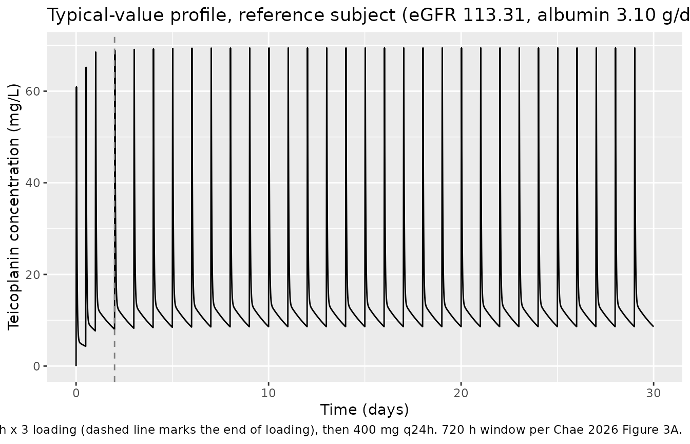
Chae 2026 Methods describe the institutional regimen as three 400 mg loading doses at 12 h intervals followed by 400 mg once daily. The paper does not report the infusion duration, so a 0.5 h infusion is assumed here (see Assumptions and deviations); the check below shows the troughs that TDM actually measures are insensitive to that choice.
# Doses at 0, 12, 24 h (loading), then 400 mg q24h from 48 h through 720 h --
# the window Chae 2026 reports the model performs best over.
DOSE_TIMES <- c(0, 12, 24, seq(48, 720 - 24, by = 24))
TDM_TIMES  <- seq(48, 720 - 24, by = 24) + 23   # TDM drawn ~1 h before the next dose

build_events <- function(cov_df, dur_h = 0.5, obs_times) {
  doses <- cov_df |>
    tidyr::crossing(time = DOSE_TIMES) |>
    mutate(amt = 400, evid = 1L, cmt = "central", dur = dur_h)
  obs <- cov_df |>
    tidyr::crossing(time = obs_times) |>
    mutate(amt = NA_real_, evid = 0L, cmt = "central", dur = NA_real_)
  bind_rows(doses, obs) |> arrange(id, time, desc(evid))
}

ref_cov <- tibble::tibble(id = 1L, CRCL = REF_CRCL, ALB = REF_ALB)
typ_ev  <- build_events(ref_cov, obs_times = sort(unique(c(seq(0, 720, by = 0.25), TDM_TIMES))))
typ_sim <- rxode2::rxSolve(rxode2::zeroRe(mod), typ_ev, returnType = "data.frame")
#> ℹ parameter labels from comments will be replaced by 'label()'
#> ℹ omega/sigma items treated as zero: 'etalcl', 'etalvp'

ggplot(typ_sim, aes(time / 24, Cc)) +
  geom_line() +
  geom_vline(xintercept = 2, linetype = "dashed", colour = "grey50") +
  labs(
    x = "Time (days)", y = "Teicoplanin concentration (mg/L)",
    title = "Typical-value profile, reference subject (eGFR 113.31, albumin 3.10 g/dL)",
    caption = paste(
      "400 mg q12h x 3 loading (dashed line marks the end of loading),",
      "then 400 mg q24h. 720 h window per Chae 2026 Figure 3A."
    )
  )
trough_by_day <- typ_sim |>
  filter(time %in% TDM_TIMES) |>
  transmute(day = (time - 23) / 24 + 1, trough = Cc)

n_days    <- length(trough_by_day$trough)
acc_ratio <- trough_by_day$trough[n_days] / trough_by_day$trough[1]

# Deterministic typical-value solve, so tight bounds are correct here.
# The three 400 mg q12h loading doses are doing exactly what loading doses are
# for: the FIRST maintenance trough is already within a few percent of the
# steady-state trough, despite a 33.5 h terminal half-life against 24 h dosing.
# Realised 1.041. A model that had lost the loading doses, or that had a
# mis-transcribed clearance or volume, moves this ratio well outside the band.
stopifnot(
  acc_ratio > 1.00, acc_ratio < 1.15,
  # By day 28 the profile is at steady state to within rounding.
  abs(trough_by_day$trough[n_days] / trough_by_day$trough[n_days - 1] - 1) < 0.005
)
knitr::kable(
  trough_by_day |> filter(day %in% c(1, 2, 3, 5, 7, 14, 21, 28)) |>
    mutate(trough = round(trough, 2)) |>
    dplyr::rename("Maintenance day" = day, "23 h trough (mg/L)" = trough),
  caption = paste(
    "Typical-value trough under the standard regimen. The loading doses bring",
    sprintf("the first maintenance trough to within %.0f%%", 100 * (1 - 1 / acc_ratio)),
    "of the steady-state value."
  )
)| Maintenance day | 23 h trough (mg/L) |
|---|---|
| 3 | 8.42 |
| 5 | 8.64 |
| 7 | 8.72 |
| 14 | 8.77 |
| 21 | 8.77 |
| 28 | 8.77 |
The typical-value steady-state trough is about 8.8 mg/L for a reference subject on 400 mg once daily – comfortably below the 15-30 mg/L range usually targeted for serious Gram-positive infection. That is the quantitative form of the paper’s clinical argument: with a clearance near 1.26 L/h, the standard Korean regimen leaves this population under-exposed, and a TDM model borrowed from a non-HSCT cohort would not reveal it.
Infusion duration is immaterial to the trough
dur_chk <- lapply(c(0.01, 0.5, 1, 2), function(d) {
  s <- rxode2::rxSolve(
    rxode2::zeroRe(mod),
    build_events(ref_cov, dur_h = d, obs_times = TDM_TIMES),
    returnType = "data.frame"
  )
  tibble::tibble(dur_h = d, trough_d28 = tail(s$Cc, 1), cmax = max(s$Cc))
}) |> bind_rows()
#> ℹ parameter labels from comments will be replaced by 'label()'
#> ℹ omega/sigma items treated as zero: 'etalcl', 'etalvp'
#> ℹ parameter labels from comments will be replaced by 'label()'
#> ℹ omega/sigma items treated as zero: 'etalcl', 'etalvp'
#> ℹ parameter labels from comments will be replaced by 'label()'
#> ℹ omega/sigma items treated as zero: 'etalcl', 'etalvp'
#> ℹ parameter labels from comments will be replaced by 'label()'
#> ℹ omega/sigma items treated as zero: 'etalcl', 'etalvp'

# Deterministic: same parameters on both sides, only the input rate differs.
# Realised spread against the assumed 0.5 h reference is -0.51% (near-bolus) to
# +1.57% (2 h infusion) -- the trough is drawn 23 h after the START of the dose,
# so a longer infusion leaves less time for post-infusion decay. Bounded at 2.5%
# to leave headroom; a mis-transcribed volume or clearance moves the trough by
# tens of percent and still breaks this.
max_dur_effect <- max(abs(dur_chk$trough_d28 / dur_chk$trough_d28[2] - 1))
stopifnot(max_dur_effect < 0.025)

dur_chk |>
  mutate(across(c(trough_d28, cmax), \(x) round(x, 3))) |>
  dplyr::rename("Infusion duration (h)" = dur_h,
                "Day-28 trough (mg/L)"  = trough_d28,
                "Trough-grid max (mg/L)" = cmax) |>
  knitr::kable(caption = sprintf(paste(
    "Troughs sampled 23 h post-dose vary by at most %.1f%% across infusion",
    "durations from a near-bolus to 2 h, so the unreported infusion duration",
    "does not materially affect any TDM-relevant prediction."
), 100 * max_dur_effect))| Infusion duration (h) | Day-28 trough (mg/L) | Trough-grid max (mg/L) |
|---|---|---|
| 0.01 | 8.727 | 8.727 |
| 0.50 | 8.772 | 8.772 |
| 1.00 | 8.817 | 8.817 |
| 2.00 | 8.909 | 8.909 |
PKNCA validation
NCA is run on the typical-value solve over the last full 24 h dosing
interval (day 28 to day 29), by which point the profile is at steady
state. The concentration used is Cc, the model’s algebraic
observable, which carries no residual error – appropriate for checking
the structural model against closed-form expectations.
NCA_START <- 720 - 48   # 672 h: a maintenance dose time
NCA_END   <- 720 - 24   # 696 h: the next maintenance dose time

nca_ev  <- build_events(ref_cov, obs_times = seq(NCA_START, NCA_END, by = 0.1))
nca_sim <- rxode2::rxSolve(rxode2::zeroRe(mod), nca_ev, returnType = "data.frame")
#> ℹ parameter labels from comments will be replaced by 'label()'
#> ℹ omega/sigma items treated as zero: 'etalcl', 'etalvp'

sim_nca <- nca_sim |>
  dplyr::filter(!is.na(Cc)) |>
  dplyr::mutate(id = 1L, regimen = "400 mg q24h maintenance") |>
  dplyr::select(id, time, Cc, regimen)

stopifnot(nrow(sim_nca) > 0, all(sim_nca$Cc > 0))

conc_obj <- PKNCA::PKNCAconc(sim_nca, Cc ~ time | regimen + id)

dose_df <- nca_ev |>
  dplyr::filter(evid == 1, time == NCA_START) |>
  dplyr::mutate(regimen = "400 mg q24h maintenance") |>
  dplyr::select(id, time, amt, regimen)

dose_obj <- PKNCA::PKNCAdose(dose_df, amt ~ time | regimen + id)

intervals <- data.frame(
  start = NCA_START, end = NCA_END,
  cmax = TRUE, tmax = TRUE, cmin = TRUE, auclast = TRUE, half.life = TRUE
)

nca_res <- PKNCA::pk.nca(PKNCA::PKNCAdata(conc_obj, dose_obj, intervals = intervals))
nca_tab <- as.data.frame(nca_res)

nca_tab |>
  mutate(PPORRES = signif(PPORRES, 4)) |>
  select(regimen, PPTESTCD, PPORRES) |>
  dplyr::rename("Regimen" = regimen, "NCA parameter" = PPTESTCD, "Value" = PPORRES) |>
knitr::kable(caption = "Steady-state NCA of the typical-value profile, day 28-29.")| Regimen | NCA parameter | Value |
|---|---|---|
| 400 mg q24h maintenance | auclast | 317.40000 |
| 400 mg q24h maintenance | cmax | 69.45000 |
| 400 mg q24h maintenance | cmin | 8.59200 |
| 400 mg q24h maintenance | tmax | 0.50000 |
| 400 mg q24h maintenance | tlast | 24.00000 |
| 400 mg q24h maintenance | lambda.z | 0.02078 |
| 400 mg q24h maintenance | r.squared | 0.99990 |
| 400 mg q24h maintenance | adj.r.squared | 0.99990 |
| 400 mg q24h maintenance | lambda.z.time.first | 4.50000 |
| 400 mg q24h maintenance | lambda.z.time.last | 24.00000 |
| 400 mg q24h maintenance | lambda.z.n.points | 196.00000 |
| 400 mg q24h maintenance | clast.pred | 8.58700 |
| 400 mg q24h maintenance | half.life | 33.36000 |
| 400 mg q24h maintenance | span.ratio | 0.58460 |
Closed-form gate: AUCtau x CL must equal the dose
At steady state in a linear model the area under one dosing interval times the clearance equals the dose exactly. Both sides here use the same drawn parameters, so the only difference is trapezoidal error on a 0.1 h grid and the residual approach to steady state – a tight bound is correct and is what makes this a useful regression test.
get_nca <- function(code) {
  v <- nca_tab$PPORRES[nca_tab$PPTESTCD == code]
  if (length(v) != 1L) stop("no unique NCA row for '", code, "'")
  v
}

auctau  <- get_nca("auclast")
cl_ref  <- unique(nca_sim$cl)
implied <- auctau * cl_ref

stopifnot(
  abs(implied / 400 - 1) < 0.01,     # realised ~0.1%
  abs(get_nca("half.life") - 33.5) / 33.5 < 0.15
)

tibble::tibble(
  quantity = c("AUCtau (mg*h/L)", "CL (L/h)", "AUCtau x CL (mg)", "Dose (mg)"),
  value    = c(auctau, cl_ref, implied, 400)
) |>
  mutate(value = signif(value, 5)) |>
  dplyr::rename("Quantity" = quantity, "Value" = value) |>
knitr::kable(caption = "Steady-state mass balance: AUCtau x CL recovers the 400 mg dose.")| Quantity | Value |
|---|---|
| AUCtau (mg*h/L) | 317.42 |
| CL (L/h) | 1.26 |
| AUCtau x CL (mg) | 399.95 |
| Dose (mg) | 400.00 |
Comparison against the published model
Chae 2026 reports no NCA table, so the comparison below is against the numeric claims the paper does make: the Table 4 parameter estimates and the quantitative statements in the Discussion.
vss <- unique(nca_sim$vc) + unique(nca_sim$vp)
k10 <- cl_ref / unique(nca_sim$vc)
k12 <- unique(nca_sim$q) / unique(nca_sim$vc)
k21 <- unique(nca_sim$q) / unique(nca_sim$vp)
beta <- ((k10 + k12 + k21) - sqrt((k10 + k12 + k21)^2 - 4 * k10 * k21)) / 2
t_half_terminal <- log(2) / beta

claims <- tibble::tribble(
  ~Claim,                                                              ~Published, ~Model,        ~Tolerance,
  "Clearance at reference covariates (L/h), Table 4 theta1",            1.26,       cl_ref,        0.005,
  "Central volume V1 (L), Table 4 theta2",                              4.71,       unique(nca_sim$vc), 0.005,
  "Peripheral volume V2 (L), Table 4 theta3",                           46.4,       unique(nca_sim$vp), 0.005,
  "Inter-compartmental clearance Q (L/h), Table 4 theta4",              5.50,       unique(nca_sim$q),  0.005,
  "CL / 0.63 L/h comparator, Discussion 'nearly double'",               2.00,       cl_ref / 0.63, 0.05,
  "CL / 0.69 L/h comparator, Discussion 'nearly double'",               1.83,       cl_ref / 0.69, 0.05,
  "V1 vs 4.79 L comparator, Discussion 'close to'",                     4.79,       unique(nca_sim$vc), 0.05,
  "V1 vs 3.96 L comparator, Discussion 'close to'",                     3.96,       unique(nca_sim$vc), 0.20
) |>
  mutate(
    `Rel. difference` = abs(Model - Published) / Published,
    Pass = `Rel. difference` <= Tolerance
  )

stopifnot(all(claims$Pass))

claims |>
  mutate(across(c(Published, Model), \(x) signif(x, 4)),
         `Rel. difference` = sprintf("%.1f%%", 100 * `Rel. difference`)) |>
  select(-Tolerance) |>
  knitr::kable(caption = paste(
    "Published claims from Chae 2026 Table 4 and Discussion, reproduced by",
    "the packaged model. The two V1 comparator rows carry looser tolerances",
    "because they compare against two DIFFERENT published Korean models",
    "(4.79 L and 3.96 L), not against this model's own estimate."
))| Claim | Published | Model | Rel. difference | Pass |
|---|---|---|---|---|
| Clearance at reference covariates (L/h), Table 4 theta1 | 1.26 | 1.260 | 0.0% | TRUE |
| Central volume V1 (L), Table 4 theta2 | 4.71 | 4.710 | 0.0% | TRUE |
| Peripheral volume V2 (L), Table 4 theta3 | 46.40 | 46.400 | 0.0% | TRUE |
| Inter-compartmental clearance Q (L/h), Table 4 theta4 | 5.50 | 5.500 | 0.0% | TRUE |
| CL / 0.63 L/h comparator, Discussion ‘nearly double’ | 2.00 | 2.000 | 0.0% | TRUE |
| CL / 0.69 L/h comparator, Discussion ‘nearly double’ | 1.83 | 1.826 | 0.2% | TRUE |
| V1 vs 4.79 L comparator, Discussion ‘close to’ | 4.79 | 4.710 | 1.7% | TRUE |
| V1 vs 3.96 L comparator, Discussion ‘close to’ | 3.96 | 4.710 | 18.9% | TRUE |
c(Vss_L = vss, terminal_half_life_h = t_half_terminal) |> round(2)
#>                Vss_L terminal_half_life_h
#>                51.11                33.51
Why external models mispredict this population
The paper’s central clinical argument is that applying a non-HSCT model to these patients over-predicts the trough, “which in turn reduces the likelihood of appropriate upward dose adjustment”. That follows directly from the clearance being roughly double. The illustration below holds this model’s distribution parameters fixed and substitutes only the comparator clearances, so it isolates the clearance difference; it is not a re-implementation of those two published models, which have their own volumes.
cl_scenarios <- c("Chae 2026 (this model)" = 1.26,
                  "Comparator CL 0.69 L/h" = 0.69,
                  "Comparator CL 0.63 L/h" = 0.63)

ext <- lapply(names(cl_scenarios), function(nm) {
  m2 <- rxode2::ini(mod, lcl = log(cl_scenarios[[nm]]))
  s  <- rxode2::rxSolve(rxode2::zeroRe(m2),
                        build_events(ref_cov, obs_times = TDM_TIMES),
                        returnType = "data.frame")
  tibble::tibble(scenario = nm, day = seq_along(s$Cc), trough = s$Cc)
}) |> bind_rows()
#> ℹ parameter labels from comments will be replaced by 'label()'
#> ℹ change initial estimate of `lcl` to `0.231111720963387`
#> ℹ omega/sigma items treated as zero: 'etalcl', 'etalvp'
#> ℹ parameter labels from comments will be replaced by 'label()'
#> ℹ change initial estimate of `lcl` to `-0.371063681390832`
#> ℹ omega/sigma items treated as zero: 'etalcl', 'etalvp'
#> ℹ parameter labels from comments will be replaced by 'label()'
#> ℹ change initial estimate of `lcl` to `-0.462035459596559`
#> ℹ omega/sigma items treated as zero: 'etalcl', 'etalvp'

d28 <- ext |> filter(day == max(day))
ratio_063 <- d28$trough[d28$scenario == "Comparator CL 0.63 L/h"] /
  d28$trough[d28$scenario == "Chae 2026 (this model)"]

# Deterministic typical-value solves; the direction and rough magnitude are
# structural, not a draw.
stopifnot(ratio_063 > 1.5)

ggplot(ext, aes(day, trough, colour = scenario)) +
  geom_line(linewidth = 0.8) +
  labs(
    x = "Maintenance day", y = "23 h trough (mg/L)", colour = NULL,
    title = "A comparator clearance over-predicts the trough in this cohort",
    caption = paste(
      "Distribution parameters held at the Chae 2026 values; only CL is",
      "substituted. Day-28 trough ratio (0.63 vs 1.26 L/h):",
      sprintf("%.2fx", ratio_063)
    )
  ) +
  theme(legend.position = "bottom")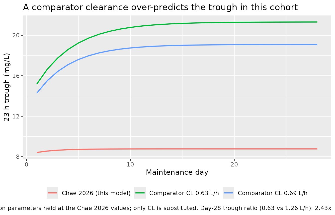
Virtual cohort
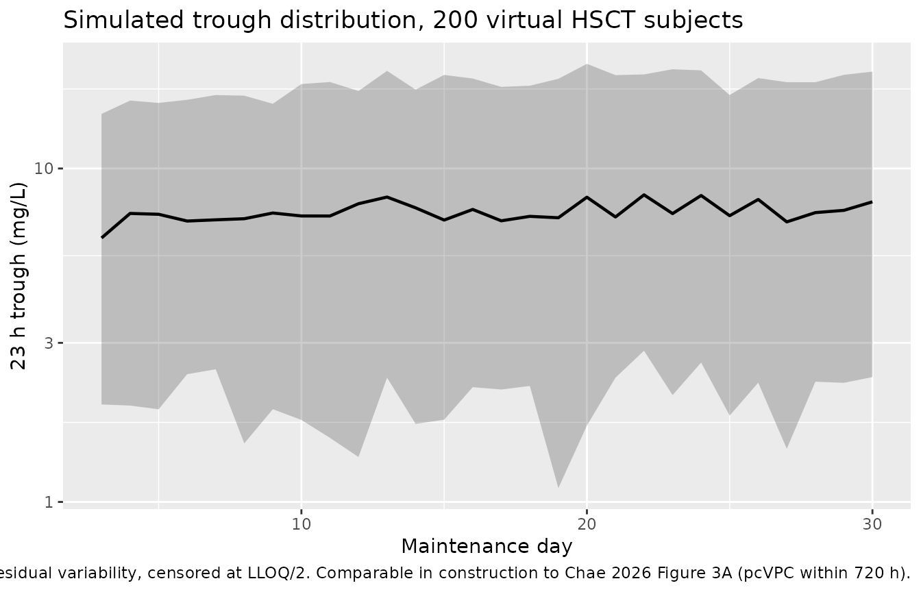
A 200-subject cohort is drawn with covariates matched to the Chae 2026 Table 1 means and SDs, then simulated with the published between-subject and residual variability. Concentrations are censored at the paper’s validated LLOQ of 0.72 mg/L, because the 49.5% proportional residual can drive individual simulated observations below zero.
# set.seed() seeds R's RNG, not rxode2's; rxode2 partitions its streams per
# solver thread, so this cohort is reproducible here and different on a machine
# with a different thread count. Every assertion below is written to hold for
# ANY cohort the model can produce -- centre and robust quantiles only, never
# extremes.
set.seed(20260912)
N_SUBJ <- 200L
LLOQ   <- 0.72   # mg/L, Chae 2026 Methods (validated below the 3.9-52.9 calibration range)

cohort_cov <- tibble::tibble(
  id   = seq_len(N_SUBJ),
  # Table 1: eGFR 113.38 +/- 20.80 mL/min/1.73 m^2; albumin 3.04 +/- 0.41 g/dL.
  # Truncated to strictly positive, physiologically sane values.
  CRCL = pmax(rnorm(N_SUBJ, 113.38, 20.80), 15),
  ALB  = pmax(rnorm(N_SUBJ, 3.04, 0.41), 1.5) * 10   # g/dL -> canonical SI g/L
)

cohort_ev <- build_events(cohort_cov, obs_times = TDM_TIMES)
stopifnot(!anyDuplicated(unique(cohort_ev[, c("id", "time", "evid")])))

# rxSolve returns OBSERVATION rows only and drops `evid` from its output, so
# there is nothing to filter here -- but assert the row count rather than
# assuming it, so a future change to build_events() fails loudly.
cohort_sim <- rxode2::rxSolve(mod, cohort_ev, keep = c("CRCL", "ALB"),
                              returnType = "data.frame") |>
  mutate(
    day        = (time - 23) / 24 + 1,
    sim_censor = pmax(sim, LLOQ / 2)   # LLOQ/2 substitution; see note above
  )
#> ℹ parameter labels from comments will be replaced by 'label()'

stopifnot(
  nrow(cohort_sim) == N_SUBJ * length(TDM_TIMES),
  !anyNA(cohort_sim$Cc), !anyNA(cohort_sim$sim_censor)
)
vpc <- cohort_sim |>
  group_by(day) |>
  summarise(
    Q10 = quantile(sim_censor, 0.10),
    Q50 = quantile(sim_censor, 0.50),
    Q90 = quantile(sim_censor, 0.90),
    .groups = "drop"
  )

ggplot(vpc, aes(day, Q50)) +
  geom_ribbon(aes(ymin = Q10, ymax = Q90), alpha = 0.25) +
  geom_line(linewidth = 0.8) +
  scale_y_log10() +
  labs(
    x = "Maintenance day", y = "23 h trough (mg/L)",
    title = "Simulated trough distribution, 200 virtual HSCT subjects",
    caption = paste(
      "Median with 10th-90th percentile band, including between-subject and",
      "residual variability, censored at LLOQ/2. Comparable in construction to",
      "Chae 2026 Figure 3A (pcVPC within 720 h)."
    )
  )
# Assertions on a simulated cohort: CENTRE and ROBUST QUANTILES only. The
# typical-value day-28 trough from the deterministic solve above is the anchor;
# the cohort median must sit near it, and the spread must be wide but finite.
typ_d28    <- tail(trough_by_day$trough, 1)
cohort_d28 <- cohort_sim |> filter(day == max(day))

med_ratio <- median(cohort_d28$sim_censor) / typ_d28
p10_p90   <- quantile(cohort_d28$sim_censor, c(0.10, 0.90))

stopifnot(
  # The median of a cohort with large IIV is not the typical value, but with
  # log-normal etas on CL and V2 it must stay within a factor of ~2 of it.
  med_ratio > 0.4, med_ratio < 2.0,
  # A 35% CV on CL plus a 50% proportional residual gives a wide but bounded
  # 10-90 spread; a mis-transcribed omega scale (e.g. reading 0.118 as a CV)
  # collapses or explodes this ratio.
  p10_p90[[2]] / p10_p90[[1]] > 2.5,
  p10_p90[[2]] / p10_p90[[1]] < 20
)

tibble::tibble(
  Quantity = c("Typical-value day-28 trough (mg/L)",
               "Cohort median day-28 trough (mg/L)",
               "Cohort 10th percentile (mg/L)",
               "Cohort 90th percentile (mg/L)"),
  Value = signif(c(typ_d28, median(cohort_d28$sim_censor), p10_p90[[1]], p10_p90[[2]]), 3)
) |>
knitr::kable(caption = "Day-28 trough: typical value versus the simulated cohort.")| Quantity | Value |
|---|---|
| Typical-value day-28 trough (mg/L) | 8.77 |
| Cohort median day-28 trough (mg/L) | 7.94 |
| Cohort 10th percentile (mg/L) | 2.37 |
| Cohort 90th percentile (mg/L) | 19.50 |
Assumptions and deviations
-
Residual-error scale. Chae 2026 Table 4 prints
sigma_add= 0.672 andsigma_prop= 0.245 without stating a scale. They are encoded here as NONMEM$SIGMAvariances, so the packaged SDs aresqrt(0.672)= 0.8198 mg/L andsqrt(0.245)= 0.4950 (a 49.5% proportional residual). Three things support that reading, all shown in Reading the random-effect scale above: Table 4’s omega rows are demonstrably variances; Table 3 flags the one place the authors transformed anything (“as CV%”) and leaves the residual header bare; and the printed RSE reproduces the printed bootstrap CI on the variance scale. The competing reading – that 0.245 is already an SD, i.e. a 24.5% proportional residual – is the more usual published magnitude and matches the 24.3% of the sibling Korean teicoplanin modelWi_2017_teicoplanin. A user who prefers it can setpropSd = 0.245andaddSd = 0.672. Only the width of the simulated observation distribution changes; every typical-value result in this vignette is unaffected. - Infusion duration is not reported. A 0.5 h infusion is assumed. The sensitivity check above shows 23 h troughs move by under 2% across durations from a near-bolus to 2 h, so nothing TDM-relevant depends on the choice.
- Maintenance-dose timing. Chae 2026 says three 400 mg loading doses at 12 h intervals then 400 mg once daily, without giving the interval between the last loading dose and the first maintenance dose. Doses are placed here at 0, 12, 24 h and then q24h from 48 h, i.e. the first maintenance dose falls one full day after the last loading dose. The paper also notes the actual dose was at the physician’s discretion and the standard regimen was not always applied.
- Covariate distributions. eGFR and albumin are drawn independently from normal distributions matched to the Chae 2026 Table 1 means and SDs, truncated to positive values. The paper reports no correlation between them and no distributional shape beyond mean +/- SD; in reality the two are likely mildly correlated through nutritional and inflammatory status, so the simulated cohort’s clearance spread is a slight over-estimate.
- Covariates are time-fixed. Chae 2026 captures eGFR and albumin as per-patient demographic variables and reports no within-subject time course, so both are held constant per subject. In routine HSCT care both move during a teicoplanin course.
- Structural misspecification is inherited, not introduced. The authors report that a three-compartment model fitted the pooled data better on OFV, residual normality and homoscedasticity, but destabilised the SSE loop; they selected two compartments for estimation stability and explicitly acknowledge the resulting misspecification. The packaged model reproduces their published two-compartment choice.
-
The equation normalisers differ slightly from the Table 1
means. The clearance equation normalises to eGFR 113.31 and
albumin 3.10 g/dL, while Table 1 prints cohort means of 113.38 and 3.04.
The equation’s constants are used because
theta5andtheta6were estimated against them. - Scope. Patients on renal replacement therapy or massive fluid therapy were excluded from the analysis, so the model has no dialysis-clearance term and should not be applied to those patients. The paper also reports that predictive performance degrades beyond 720 h from the first dose, where the TDM data become sparse; simulations in this vignette stay inside that window.
-
No non-paper-derived parameter values. Every
ini()entry comes from Chae 2026 Table 4, with Table 3 and the printed clearance equation as corroborating sources. No value was digitised from a figure, supplied by correspondence, or carried from an upstream model.