Berzosertib (Terranova 2021)

Model and source

#> ℹ parameter labels from comments will be replaced by 'label()'

• Citation: Terranova N, Jansen M, Falk M, Hendriks BS. Population pharmacokinetics of ATR inhibitor berzosertib in phase I studies for different cancer types. Cancer Chemother Pharmacol. 2021;87(2):185-196. doi:10.1007/s00280-020-04184-z. Structural and random-effect estimates from Table 3; covariate coefficients recovered from the numeric ratios printed in the Figure 2 forest plots.

• Description: Two-compartment population PK model (full covariate model) for intravenous berzosertib (M6620, VX-970), an ATR inhibitor, in adults with advanced solid tumors receiving 1-h infusions alone or combined with gemcitabine, cisplatin, carboplatin, or carboplatin plus paclitaxel. Linear elimination; a full 4x4 IIV block on CL, V1, Q and V2; combined additive plus proportional residual error. Body weight, age, albumin, platelet count and baseline tumor size (power, centred on the cohort medians) and sex, hepatic impairment, renal impairment, ECOG 0 and tumor type (NSCLC, TNBC, CRC; linear) act on CL, V1 and V2.

• Article (open access): https://doi.org/10.1007/s00280-020-04184-z

• Online Resource (Figures S1-S5, Tables S1-S2): https://static-content.springer.com/esm/art%3A10.1007%2Fs00280-020-04184-z/MediaObjects/280_2020_4184_MOESM1_ESM.docx

Berzosertib (M6620, formerly VX-970) is an intravenous first-in-class inhibitor of the ataxia-telangiectasia and Rad3-related (ATR) kinase, developed in combination with DNA-damaging chemotherapy. Terranova 2021 pooled two phase I studies and described berzosertib plasma concentrations with a linear two-compartment model. Covariates were handled with a full covariate model: every pre-specified covariate was estimated on CL, V1 and V2 simultaneously and all were kept, whether or not the effect was clinically relevant. The paper’s final model is therefore the full covariate model, whose structural and random-effect estimates are in Table 3.

Population

The analysis used 2546 plasma concentrations from 240 adults with advanced solid tumors (Study 001, MS201923-0001 / NCT02157792, n = 170; Study 002, VX13-970-002 / EudraCT 2013-005100-34, n = 70). Berzosertib was given as 1-h intravenous infusions of 18-480 mg/m^2 (11 dose levels), either alone (once or twice weekly) or on days 2 and 9 of 21-day cycles after gemcitabine, cisplatin, gemcitabine plus cisplatin, carboplatin, or carboplatin plus paclitaxel (Terranova 2021 Table 1).

Baseline characteristics (Terranova 2021 Table 2): median age 60 years (26-79), median weight 72.8 kg (46-150), median BSA 1.82 m^2 (1.4-2.59), 60.4% female, 93.3% White. Tumor types were NSCLC 20.0%, CRC 18.3%, TNBC 13.8%, SCLC 6.7%, mesothelioma 5.0%, non-TNBC breast 4.6%, ovarian 3.8%, prostate 2.9%, head and neck 0.4% and other 24.6%. Mild or moderate renal impairment was present in 43% and mild or severe hepatic impairment in 18%, and 27% had ECOG PS 0.

str(ui$population)
#> List of 15
#>  $ species       : chr "human"
#>  $ n_subjects    : int 240
#>  $ n_studies     : int 2
#>  $ n_observations: int 2546
#>  $ age_range     : chr "26-79 years"
#>  $ age_median    : chr "60 years"
#>  $ weight_range  : chr "46-150 kg"
#>  $ weight_median : chr "72.8 kg"
#>  $ bsa_median    : chr "1.82 m^2 (range 1.4-2.59)"
#>  $ sex_female_pct: num 60.4
#>  $ race_ethnicity: Named num [1:5] 93.3 1.25 2.08 2.5 0.83
#>   ..- attr(*, "names")= chr [1:5] "White" "Black" "Asian" "Other" ...
#>  $ disease_state : chr "Advanced solid tumors (and DDR-defective lymphoma in Study 002 Part C): NSCLC 20.0%, CRC 18.3%, TNBC 13.8%, SCL"| __truncated__
#>  $ dose_range    : chr "Berzosertib 18-480 mg/m^2 as 1-h IV infusions (11 dose levels), alone (once or twice weekly) or on days 2 and 9"| __truncated__
#>  $ regions       : chr "Two phase I studies: Study 001 (MS201923-0001, NCT02157792; n = 170) and Study 002 (VX13-970-002, EudraCT 2013-"| __truncated__
#>  $ notes         : chr "Baseline characteristics from Terranova 2021 Table 2. Renal impairment none 57.1% / mild 36.7% / moderate 6.25%"| __truncated__

Source trace

Every ini() entry in inst/modeldb/specificDrugs/Terranova_2021_berzosertib.R carries an in-file comment naming its source location.

Equation / parameter	Value	Source location
Structure: 2-cmt, linear elimination, 1-h IV infusion	–	Results ‘Base model’; Methods ‘Clinical trials’
lcl (CL)	65 L/h	Table 3
lvc (V1)	118 L	Table 3
lq (Q)	295 L/h	Table 3
lvp (V2)	1030 L	Table 3
Categorical form P = theta1 * (1 + thetak * CAT)	–	Methods ‘Covariate analysis model development’
Continuous form P = theta1 * (CON / CON_median)^theta2	–	Methods ‘Covariate analysis model development’
Centring medians WT 72.8 kg, AGE 60 y, ALB 38 g/L, PLT 274 x 10^9/L, TUMSZ 75 mm	–	Table 2
e_wt_*, e_age_*, e_alb_*, e_plt_*, e_tumsz_* (15 power exponents)	see ini()	Back-solved from the two printed Figure 2 ratios per covariate (see below)
e_sexf_*, e_hepimp_*, e_renalimp_*, e_ecog0_*, e_tumtp_* (21 linear effects)	printed ratio - 1	Figure 2A-C printed ratios
etalcl + etalvc + etalq + etalvp block	variances 0.066, 0.32, 0.24, 0.047	Table 3 (IIV and cov rows)
propSd	0.22	Table 3
addSd	1.73 ng/mL	Table 3
Cc = 1000 * central / vc	ng/mL	Dose in mg, volumes in L; concentrations in ng/mL (LLOQ 10 ng/mL)

Recovering the covariate coefficients from Figure 2

The paper prints no table of covariate coefficients. Figure 2 does print, for every covariate, the median ratio of the parameter at a covariate value to the typical value, with its 95% CI. For categorical covariates that ratio is 1 + theta directly. For continuous covariates each covariate appears at two values (its 2.5th and 97.5th percentiles), and under the power model ratio = (x / median)^theta, so

theta = log(r_high / r_low) / log(x_high / x_low),

which uses only printed numbers and does not depend on the centring median. The check below goes the other way. It rebuilds every Figure 2 ratio from the encoded model, using the Table 2 medians as the centring values, and compares each with the printed value.

p <- ui$theta
fig2 <- tribble(
  ~param, ~cov, ~x, ~printed,
  "cl", "wt", 51, 0.911, "cl", "wt", 114, 1.12,
  "cl", "age", 35, 1.05, "cl", "age", 76, 0.977,
  "cl", "alb", 26, 0.921, "cl", "alb", 46, 1.04,
  "cl", "plt", 132, 1.1, "cl", "plt", 551, 0.911,
  "cl", "tumsz", 17, 0.997, "cl", "tumsz", 201, 1,
  "vc", "wt", 51, 1.05, "vc", "wt", 114, 0.947,
  "vc", "age", 35, 0.979, "vc", "age", 76, 1.01,
  "vc", "alb", 26, 0.714, "vc", "alb", 46, 1.18,
  "vc", "plt", 115, 1.13, "vc", "plt", 565, 0.891,
  "vc", "tumsz", 17, 0.727, "vc", "tumsz", 201, 1.24,
  "vp", "wt", 51, 0.96, "vp", "wt", 114, 1.05,
  "vp", "age", 35, 0.833, "vp", "age", 76, 1.08,
  "vp", "alb", 26, 0.906, "vp", "alb", 46, 1.05,
  "vp", "plt", 115, 1.04, "vp", "plt", 565, 0.964,
  "vp", "tumsz", 17, 0.99, "vp", "tumsz", 201, 1.01
)
med <- c(wt = 72.8, age = 60, alb = 38, plt = 274, tumsz = 75)
fig2 <- fig2 |>
  mutate(
    model = (x / med[cov])^p[paste0("e_", cov, "_", param)],
    abs_diff = abs(model - printed)
  )
knitr::kable(fig2, digits = 3)

param	cov	x	printed	model	abs_diff
cl	wt	51	0.911	0.913	0.002
cl	wt	114	1.120	1.122	0.002
cl	age	35	1.050	1.051	0.001
cl	age	76	0.977	0.978	0.001
cl	alb	26	0.921	0.922	0.001
cl	alb	46	1.040	1.042	0.002
cl	plt	132	1.100	1.101	0.001
cl	plt	551	0.911	0.912	0.001
cl	tumsz	17	0.997	0.998	0.001
cl	tumsz	201	1.000	1.001	0.001
vc	wt	51	1.050	1.047	0.003
vc	wt	114	0.947	0.944	0.003
vc	age	35	0.979	0.979	0.000
vc	age	76	1.010	1.010	0.000
vc	alb	26	0.714	0.716	0.002
vc	alb	46	1.180	1.183	0.003
vc	plt	115	1.130	1.138	0.008
vc	plt	565	0.891	0.898	0.007
vc	tumsz	17	0.727	0.726	0.001
vc	tumsz	201	1.240	1.237	0.003
vp	wt	51	0.960	0.961	0.001
vp	wt	114	1.050	1.051	0.001
vp	age	35	0.833	0.835	0.002
vp	age	76	1.080	1.082	0.002
vp	alb	26	0.906	0.906	0.000
vp	alb	46	1.050	1.051	0.001
vp	plt	115	1.040	1.042	0.002
vp	plt	565	0.964	0.966	0.002
vp	tumsz	17	0.990	0.988	0.002
vp	tumsz	201	1.010	1.008	0.002

Every ratio is reproduced to within 0.008. That residual comes from the three-significant-figure rounding of the printed ratios, which the exponent inherits, and from the percentiles being printed as rounded covariate values. The largest gaps are for platelets on V1. There the two printed ratios imply a centring value of about 260 x 10^9/L rather than the Table 2 median of 274.

stopifnot(
  # Deterministic (no random draws). A wrong exponent sign, a swapped CL/V1
  # row, or a wrong centring median moves a ratio by far more than rounding.
  max(fig2$abs_diff) < 0.012,
  median(fig2$abs_diff) < 0.005
)

Which sex is the reference category?

The Methods state that the categorical indicator is 0 for the most common category, which for sex would be female (60.4%). Figure 2, however, plots the effect for ‘Sex: Female’, and the Results state that V1 in females is 15.8% lower than in males. Figure 2 plots the indicator category for every other covariate (hepatic and renal impairment, ECOG 0, the three tumor types). So the figure implies female is the indicator and the Table 3 typical values refer to a male.

These two readings can be told apart, because the base model (no covariates, Online Resource Table S2) estimates the population typical value directly. Under the correct reading, the full-model typical values, averaged over the cohort’s categorical covariates, should come close to the base-model estimates. The continuous covariates are centred on their medians and contribute little. The calculation below uses the Table 2 category frequencies. Missing hepatic status is counted as normal, as in the paper.

freq <- c(male = 95 / 240, hepimp = 44 / 240, renalimp = 103 / 240, ecog0 = 65 / 240,
          nsclc = 48 / 240, tnbc = 33 / 240, crc = 44 / 240)
ratio <- function(par, what) 1 + p[paste0("e_", what, "_", par)]
logshift_other <- function(par) {
  freq[["hepimp"]] * log(ratio(par, "hepimp")) +
    freq[["renalimp"]] * log(ratio(par, "renalimp")) +
    freq[["ecog0"]] * log(ratio(par, "ecog0")) +
    freq[["nsclc"]] * log(ratio(par, "tumtp_nsclc")) +
    freq[["tnbc"]] * log(ratio(par, "tumtp_tnbc")) +
    freq[["crc"]] * log(ratio(par, "tumtp_crc"))
}
tv <- c(cl = 65, vc = 118, vp = 1030)       # Table 3
base <- c(cl = 56, vc = 111, vp = 861)      # Online Resource Table S2
adjud <- data.frame(parameter = names(tv), base_model = base) |>
  mutate(
    # Male reference: females (1 - freq male) carry the Figure 2 ratio.
    male_reference = tv * exp((1 - freq[["male"]]) * log(sapply(parameter, ratio, what = "sexf")) +
                               sapply(parameter, logshift_other)),
    # Female reference: males carry the inverse of the Figure 2 ratio.
    female_reference = tv * exp(-freq[["male"]] * log(sapply(parameter, ratio, what = "sexf")) +
                                 sapply(parameter, logshift_other))
  )
knitr::kable(adjud, digits = 1, row.names = FALSE)

parameter	base_model	male_reference	female_reference
cl	56	60.1	68.4
vc	111	117.8	140.0
vp	861	843.8	980.0

stopifnot(all(abs(log(adjud$male_reference / adjud$base_model)) <
                abs(log(adjud$female_reference / adjud$base_model))))

The male-reference reading comes within 2-8% of the base-model estimate for all three parameters. The female-reference reading overshoots by 14-26%. The model therefore uses SEXF as the indicator, (1 + e_sexf_<param> * SEXF), with Table 3 describing a male.

Virtual cohort

Individual covariates are not available. The Figure 3 simulations resampled covariate vectors jointly from the study data, so the cohort below is built from the Table 2 marginal distributions instead. Continuous covariates are drawn independently and redrawn when they fall outside the observed range. Tumor type follows the Table 2 frequencies, TNBC patients are all female, and the other tumor types are female often enough to keep the overall 60.4%. The mg dose is the mg/m^2 dose level times the Mosteller BSA, which uses a sex-specific height.

set.seed(20210201)
n_per_arm <- 200

rtrunc <- function(n, draw, lo, hi) {
  out <- draw(n)
  bad <- out < lo | out > hi
  while (any(bad)) {
    out[bad] <- draw(sum(bad))
    bad <- out < lo | out > hi
  }
  out
}

make_cohort <- function(n) {
  tumor <- sample(c("NSCLC", "TNBC", "CRC", "Other"), n, replace = TRUE,
                  prob = c(48, 33, 44, 115))
  p_female_nontnbc <- (145 - 33) / (240 - 33)
  sexf <- ifelse(tumor == "TNBC", 1L, rbinom(n, 1, p_female_nontnbc))
  height <- ifelse(sexf == 1, rnorm(n, 162, 7), rnorm(n, 175, 7))
  data.frame(
    SEXF = sexf,
    WT = rtrunc(n, function(k) exp(rnorm(k, log(72.8), 0.2)), 46, 150),
    AGE = rtrunc(n, function(k) rnorm(k, 60, 10.5), 26, 79),
    ALB = rtrunc(n, function(k) rnorm(k, 38, 4.5), 23, 49),
    PLT = rtrunc(n, function(k) exp(rnorm(k, log(274), 0.35)), 93, 816),
    TUMSZ = rtrunc(n, function(k) exp(rnorm(k, log(75), 0.65)), 10, 312),
    HEPIMP = rbinom(n, 1, 44 / 240),
    RENALIMP = rbinom(n, 1, 103 / 240),
    ECOG_GE1 = rbinom(n, 1, 1 - 65 / 240),
    TUMTP_NSCLC = as.integer(tumor == "NSCLC"),
    TUMTP_TNBC = as.integer(tumor == "TNBC"),
    TUMTP_CRC = as.integer(tumor == "CRC"),
    height = height
  ) |>
    mutate(BSA = sqrt(height * WT / 3600))
}

cohort <- make_cohort(n_per_arm)
summary(cohort[, c("WT", "AGE", "ALB", "PLT", "TUMSZ", "BSA")])
#>        WT              AGE             ALB             PLT       
#>  Min.   : 47.33   Min.   :31.22   Min.   :28.15   Min.   :112.0  
#>  1st Qu.: 65.06   1st Qu.:52.52   1st Qu.:34.90   1st Qu.:227.7  
#>  Median : 75.74   Median :59.48   Median :37.65   Median :274.1  
#>  Mean   : 76.38   Mean   :59.15   Mean   :38.03   Mean   :298.6  
#>  3rd Qu.: 85.24   3rd Qu.:66.77   3rd Qu.:41.16   3rd Qu.:358.0  
#>  Max.   :128.84   Max.   :78.93   Max.   :48.93   Max.   :716.1  
#>      TUMSZ             BSA       
#>  Min.   : 14.24   Min.   :1.452  
#>  1st Qu.: 53.55   1st Qu.:1.728  
#>  Median : 79.54   Median :1.872  
#>  Mean   : 90.63   Mean   :1.874  
#>  3rd Qu.:117.58   3rd Qu.:2.004  
#>  Max.   :265.91   Max.   :2.448
colMeans(cohort[, c("SEXF", "HEPIMP", "RENALIMP", "ECOG_GE1", "TUMTP_NSCLC", "TUMTP_TNBC", "TUMTP_CRC")])
#>        SEXF      HEPIMP    RENALIMP    ECOG_GE1 TUMTP_NSCLC  TUMTP_TNBC 
#>       0.600       0.170       0.460       0.745       0.200       0.130 
#>   TUMTP_CRC 
#>       0.195

Simulation

Figure 3 simulated a single 1-h infusion at the three recommended phase II dose levels: 90 mg/m^2 (with carboplatin), 140 mg/m^2 (with cisplatin) and 210 mg/m^2 (with gemcitabine). The same covariate cohort is used in every arm, and each arm draws its own random effects.

arms <- data.frame(treatment = c("90 mg/m^2", "140 mg/m^2", "210 mg/m^2"),
                   dose_m2 = c(90, 140, 210))
obs_times <- sort(unique(c(seq(0, 48, by = 0.1), seq(49, 72, by = 1))))

events <- bind_rows(lapply(seq_len(nrow(arms)), function(a) {
  cov <- cohort |>
    mutate(id = (a - 1) * n_per_arm + row_number(),
           treatment = arms$treatment[a],
           dose_mg = arms$dose_m2[a] * BSA)
  dose <- cov |> mutate(time = 0, evid = 1, amt = dose_mg, rate = dose_mg, cmt = "central")
  obs <- cov |>
    select(-dose_mg) |>
    tidyr::crossing(time = obs_times) |>
    left_join(select(cov, id, dose_mg), by = "id") |>
    mutate(evid = 0, amt = 0, rate = 0, cmt = "central")
  bind_rows(dose, obs)
})) |>
  arrange(id, time, desc(evid))

rxode2::rxSetSeed(20210201)
sim <- rxode2::rxSolve(ui, events, keep = c("treatment", "dose_mg")) |>
  as.data.frame() |>
  mutate(treatment = factor(treatment, levels = arms$treatment))

ic50 <- 110
sim |>
  filter(time >= 0.1) |>
  group_by(treatment, time) |>
  summarise(med = median(Cc), lo = quantile(Cc, 0.05), hi = quantile(Cc, 0.95), .groups = "drop") |>
  ggplot(aes(time, med, colour = treatment, fill = treatment)) +
  geom_ribbon(aes(ymin = lo, ymax = hi), alpha = 0.15, colour = NA) +
  geom_line() +
  geom_hline(yintercept = ic50, linetype = "dashed") +
  scale_y_log10() +
  coord_cartesian(xlim = c(0, 48), ylim = c(10, NA)) +
  labs(x = "Time after start of infusion (h)", y = "Berzosertib (ng/mL)",
       colour = NULL, fill = NULL)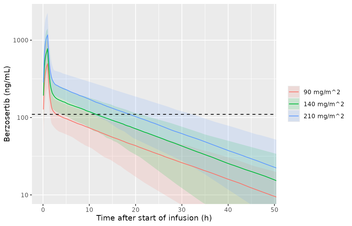

Simulated berzosertib concentrations after a single 1-h infusion (median and 5th-95th percentiles). Dashed line: p-Chk1 IC50 of 110 ng/mL (Terranova 2021).

Replicating Figure 3 and the IC50 statistics

Terranova 2021 reports the mean Cmax/IC50 ratio (4.8, 7.5 and 11.2 at 90, 140 and 210 mg/m^2) and the mean time above IC50 with a 95% CI: 2.5 h (1-8 h), 8 h (2-20 h) and 16 h (8-28 h). It also reports the percentage of subjects whose average concentration exceeded IC50: 54%, 91% and 99%.

dt <- diff(obs_times)
ind <- sim |>
  group_by(treatment, id) |>
  arrange(time, .by_group = TRUE) |>
  summarise(
    cmax = max(Cc),
    # Time above IC50 on the 0.1-h grid (the concentration falls below IC50
    # well before 48 h at every dose, where the grid coarsens).
    t_above = sum((Cc[-n()] > ic50) * diff(time)),
    cavg12 = sum(((Cc[-n()] + Cc[-1]) / 2 * diff(time))[time[-1] <= 12]) / 12,
    cavg24 = sum(((Cc[-n()] + Cc[-1]) / 2 * diff(time))[time[-1] <= 24]) / 24,
    cl = cl[1],
    dose_mg = dose_mg[1],
    .groups = "drop"
  )

ind |>
  select(treatment, id, Cmax = cmax, Cavg = cavg12) |>
  pivot_longer(c(Cmax, Cavg)) |>
  mutate(name = factor(name, c("Cmax", "Cavg"))) |>
  ggplot(aes(treatment, value)) +
  geom_boxplot() +
  geom_hline(yintercept = ic50, linetype = "dashed", colour = "blue") +
  facet_wrap(~name, scales = "free_y") +
  labs(x = NULL, y = "Berzosertib (ng/mL)")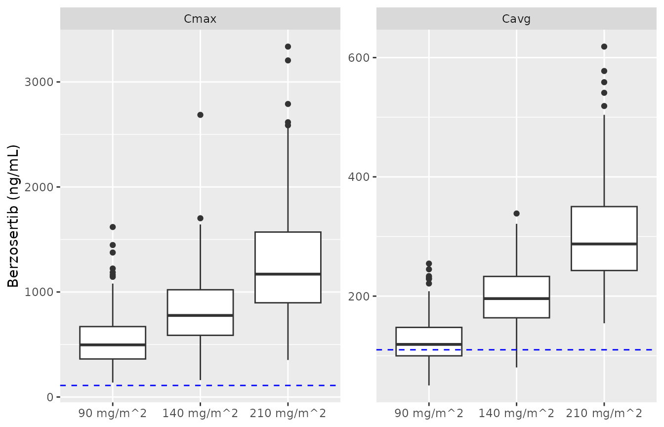

Replicates Figure 3 of Terranova 2021: distributions of simulated Cmax (left) and Cavg (right; 0-12 h window, see text) after a single dose. Dashed line: p-Chk1 IC50.

pub <- data.frame(
  treatment = arms$treatment,
  cmax_ic50_pub = c(4.8, 7.5, 11.2),
  t_above_pub = c(2.5, 8, 16),
  t_above_lo_pub = c(1, 2, 8),
  t_above_hi_pub = c(8, 20, 28),
  pct_cavg_pub = c(54, 91, 99)
)
fig3_tab <- ind |>
  group_by(treatment) |>
  summarise(
    cmax_ic50_sim = mean(cmax) / ic50,
    t_above_median_sim = median(t_above),
    t_above_mean_sim = mean(t_above),
    t_above_p2.5_sim = quantile(t_above, 0.025),
    t_above_p97.5_sim = quantile(t_above, 0.975),
    pct_cavg12_sim = 100 * mean(cavg12 > ic50),
    pct_cavg24_sim = 100 * mean(cavg24 > ic50)
  ) |>
  left_join(pub, by = "treatment")
fig3_tab |>
  select(treatment, cmax_ic50_pub, cmax_ic50_sim, t_above_pub, t_above_median_sim,
         t_above_mean_sim, t_above_lo_pub, t_above_p2.5_sim, t_above_hi_pub,
         t_above_p97.5_sim, pct_cavg_pub, pct_cavg12_sim, pct_cavg24_sim) |>
  knitr::kable(digits = 2)

treatment	cmax_ic50_pub	cmax_ic50_sim	t_above_pub	t_above_median_sim	t_above_mean_sim	t_above_lo_pub	t_above_p2.5_sim	t_above_hi_pub	t_above_p97.5_sim	pct_cavg_pub	pct_cavg12_sim	pct_cavg24_sim
90 mg/m^2	4.8	5.00	2.5	2.80	4.11	1	1.20	8	12.92	54	63.0	18.5
140 mg/m^2	7.5	7.47	8.0	11.35	11.70	2	2.20	20	23.40	91	98.5	79.5
210 mg/m^2	11.2	11.49	16.0	18.65	19.52	8	9.39	28	33.40	99	100.0	99.5

The mean Cmax/IC50 ratio is reproduced at all three doses (simulated 5.0, 7.5, 11.5).

Time above IC50 comes out somewhat longer in the simulation than published. The lower 2.5th percentiles match the published lower 95% bounds (1.2, 2.2, 9.4 h versus 1, 2 and 8 h). The simulated medians (2.8, 11.4, 18.6 h) and upper 97.5th percentiles (12.9, 23.4, 33.4 h) lie above the published point values (2.5, 8 and 16 h) and upper bounds (8, 20 and 28 h). The published values are round numbers that look like they were read off a coarse time grid, which would shorten the measured time above IC50. The paper calls them ‘mean’ times, but the simulated mean is further still from them at 90 mg/m^2. Cmax, and so the covariate and random-effect structure that sets it, is reproduced. The discrepancy is therefore attributed to how time above IC50 was measured, not to the model.

The paper does not define the averaging window for Cavg. With a 12-h window the percentage of simulated subjects whose Cavg exceeds IC50 is 63%, 98%, 100%. With a 24-h window it is 18%, 80%, 100%. The published 54%, 91% and 99% lie between the two and closer to the 12-h values, so Figure 3 is replicated with a 12-h window. This window is inferred from the numbers; the paper does not state it.

stopifnot(
  # Mean Cmax is set by dose / V1 and CL; the IIV on V1 is large (0.32), so
  # allow 15% for the cohort draw.
  all(abs(fig3_tab$cmax_ic50_sim / fig3_tab$cmax_ic50_pub - 1) < 0.15),
  # The median time above IC50 lies inside the published 95% interval.
  all(fig3_tab$t_above_median_sim > fig3_tab$t_above_lo_pub &
        fig3_tab$t_above_median_sim < fig3_tab$t_above_hi_pub)
)

PKNCA validation

The paper has no NCA table. Single-dose NCA per arm checks two model-implied identities. First, AUC0-inf * CL = Dose, using each subject’s own clearance. Second, dose proportionality, since the model is linear.

sim_nca <- sim |>
  filter(!is.na(Cc)) |>
  select(id, time, Cc, treatment) |>
  as.data.frame()
dose_df <- events |>
  filter(evid == 1) |>
  select(id, time, amt, treatment) |>
  as.data.frame()

conc_obj <- PKNCA::PKNCAconc(sim_nca, Cc ~ time | treatment + id,
                             concu = "ng/mL", timeu = "h")
dose_obj <- PKNCA::PKNCAdose(dose_df, amt ~ time | treatment + id, doseu = "mg")
intervals <- data.frame(start = 0, end = Inf, cmax = TRUE, tmax = TRUE,
                        aucinf.obs = TRUE, half.life = TRUE)
nca_res <- PKNCA::pk.nca(PKNCA::PKNCAdata(conc_obj, dose_obj, intervals = intervals))

nca_wide <- as.data.frame(nca_res$result) |>
  filter(PPTESTCD %in% c("cmax", "tmax", "aucinf.obs", "half.life")) |>
  select(treatment, id, PPTESTCD, PPORRES) |>
  pivot_wider(names_from = PPTESTCD, values_from = PPORRES) |>
  mutate(treatment = factor(treatment, levels = arms$treatment))

nca_wide |>
  group_by(treatment) |>
  summarise(across(c(cmax, tmax, aucinf.obs, half.life), median)) |>
  rename("Dose level" = treatment, "Cmax (ng/mL)" = cmax, "Tmax (h)" = tmax,
         "AUC0-inf (ng*h/mL)" = aucinf.obs, "t1/2 (h)" = half.life) |>
  knitr::kable(digits = 1)

Dose level	Cmax (ng/mL)	Tmax (h)	AUC0-inf (ng*h/mL)	t1/2 (h)
90 mg/m^2	496.5	1	2734.1	13.3
140 mg/m^2	776.6	1	4469.4	13.7
210 mg/m^2	1170.0	1	6416.9	13.5

chk <- nca_wide |>
  inner_join(select(ind, id, cl, dose_mg), by = "id") |>
  mutate(
    # AUC in ng*h/mL; 1 ng/mL = 1e-3 mg/L, so dose (mg) = CL (L/h) * AUC / 1000.
    pct_diff = 100 * (cl * aucinf.obs / 1000 - dose_mg) / dose_mg,
    auc_per_mg = aucinf.obs / dose_mg
  )
chk |>
  group_by(treatment) |>
  summarise(median_pct_diff = median(pct_diff),
            p90_abs_pct_diff = quantile(abs(pct_diff), 0.9),
            median_auc_per_mg = median(auc_per_mg)) |>
  knitr::kable(digits = 2)

treatment	median_pct_diff	p90_abs_pct_diff	median_auc_per_mg
90 mg/m^2	-0.03	0.07	16.08
140 mg/m^2	-0.02	0.05	16.89
210 mg/m^2	-0.03	0.05	16.35

stopifnot(
  # Same drawn parameters on both sides: the gap is only trapezoid and
  # lambda-z extrapolation error, so a tight bound is appropriate.
  abs(median(chk$pct_diff)) < 2,
  quantile(abs(chk$pct_diff), 0.9) < 5
)

Comparison against the published exposure summary

The only published exposure numbers are the mean Cmax values implied by the Cmax/IC50 ratios (ratio x 110 ng/mL). Since the paper reports means, the simulated per-arm means are passed to ncaComparisonTable().

sim_mean <- nca_wide |>
  group_by(treatment) |>
  summarise(cmax = mean(cmax)) |>
  as.data.frame()
ref <- data.frame(treatment = arms$treatment, cmax = c(4.8, 7.5, 11.2) * ic50)
tbl <- nlmixr2lib::ncaComparisonTable(sim_mean, ref, by = "treatment",
                                      units = c(cmax = "ng/mL"))
knitr::kable(tbl)

NCA parameter	treatment	Reference	Simulated	% diff
Cmax (ng/mL)	90 mg/m^2	528	550	+4.1%
Cmax (ng/mL)	140 mg/m^2	825	822	-0.4%
Cmax (ng/mL)	210 mg/m^2	1230	1260	+2.6%

Assumptions and deviations

• Covariate coefficients come from Figure 2. The paper does not tabulate the full-covariate-model coefficients. Categorical effects are the printed Figure 2 ratio minus one. Continuous exponents are back-solved from the two printed ratios per covariate (see “Recovering the covariate coefficients”). The Figure 2 ratios are medians over the parameter-uncertainty distribution, which equal the point-estimate ratios for these monotone transforms. Rounding of the printed ratios to three significant figures carries into the exponents. It matters most for the near-null effects, for example tumor size on CL, whose ratios are 0.997 and 1.
• Sex reference category. The Methods say the most common category (female) is the reference. Figure 2 plots ‘Sex: Female’ as the effect category, and the base-model typical values agree with the male-reference reading (see above), so the Table 3 typical values are taken to describe a male.
• Composite categories. Hepatic impairment ‘Mild/Severe’ (NCI ODWG; no moderate cases) is encoded as HEPIMP (any impairment). Renal impairment ‘Mild/Moderate’ (FDA guidance; no severe cases) is encoded as RENALIMP. The paper compared ECOG 0 against ECOG 1, with ECOG >= 2 folded into ECOG 1, so ECOG enters as (1 - ECOG_GE1). Tumor types without their own indicator (SCLC, prostate, non-TNBC breast, head and neck, ovarian, mesothelioma, other) form the reference. Missing covariates were imputed to the median or most common category in the paper, and users should do the same.
• Residual error. Table 3 gives a proportional SD and an additive SD with no statement on how they combine. The nlmixr2 default (variances add, add() + prop()) is used. The additive term (1.73 ng/mL) is small against the 10 ng/mL LLOQ, so the choice has no practical effect.
• Table 3 typographical errors. The 95% CI printed for cov(Q, V2) (0.021-0.087) repeats the cov(CL, Q) row and does not match its estimate (0.090, RSE 16%). In Online Resource Table S2 the last variance row is labelled ‘IIV on Q’ but is the IIV on V2. Neither affects an encoded value.
• Virtual cohort. Covariates are drawn independently from the Table 2 marginals rather than resampled jointly from subject data. Body weight is not sex-specific, and height, which is used only for the Mosteller BSA, is assumed.
• Cavg window. The averaging window for Cavg in Figure 3 is not stated. The published percentages lie between the 12-h and 24-h results and closer to the 12-h ones, so the Figure 3 replication uses a 12-h window.
• Time above IC50. The simulated time above IC50 is longer than the published values (see the Figure 3 section). This is attributed to how the paper measured it, since Cmax is reproduced. The model was not adjusted.
• Base model. The paper’s base model (Online Resource Table S2) is not packaged. It is used here only to decide the sex reference category.